Post 10 — The most important mixed-model lesson was not about random effects
A common way of introducing mixed models is to start listing random effects.
Random intercepts. Random slopes. Batch. Analyst. Instrument.
But I think the more useful starting point is simpler:
Which observations are actually independent?
In this dataset we have 60 samples, each measured with four analytical methods.
A random-intercept model,
RelativeBias_pct ~ Method * Matrix + (1 | SampleID)
allows each sample to have its own baseline level of relative bias.
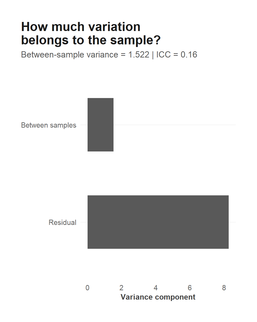
The fitted model estimates a between-sample variance of about 1.522, with an ICC of approximately 0.15.
So around 15% of the modelled variance is associated with differences between samples.
That is not evidence that the remaining 85% is “measurement error”. It is simply the residual variation after accounting for the fixed effects and the sample-level effect.
Still, the result is scientifically informative.
The sample-to-sample component is not negligible.
The model is telling us that samples differ systematically in their baseline response, while Method and Matrix explain additional structure.
And this also clarifies something about experimental design.
The four aliquots from each sample were prepared independently for the four methods. That supports treating the analytical measurements as distinct observations conditional on the sample, but it does not make the four measurements independent in the statistical sense: they still share the same sample.
The mixed model represents exactly that dependence.
I also tried a more ambitious random-slope structure, allowing the Method effect to vary by SampleID.
It failed.
Not because mixed models are unreliable, but because the dataset contains only four observations per sample. There simply is not enough within-sample information to estimate that much sample-specific structure.
Batch and Day were more interesting.
They are not nested under SampleID: the four measurements from a sample can occur in different batches and on different days. They are therefore different sources of analytical variation. Including them as fixed nuisance effects in a sensitivity analysis leaves the Method estimates broadly similar.
Analyst and Instrument have only 3 and 2 levels respectively, so treating them as random effects would add complexity without much information.
The final lesson is therefore not:
“Mixed models are more sophisticated.”
It is:
the statistical model should reflect the experimental design, and complexity should stop where the data stop supporting it.
That is probably the most useful lesson I am taking away from the whole series.
The implementation details and reproducible analysis for this step are available in the GitHub repository at https://github.com/andreabz/analytical-anova/ and on the project page at https://andreabz.github.io/analytical-anova/