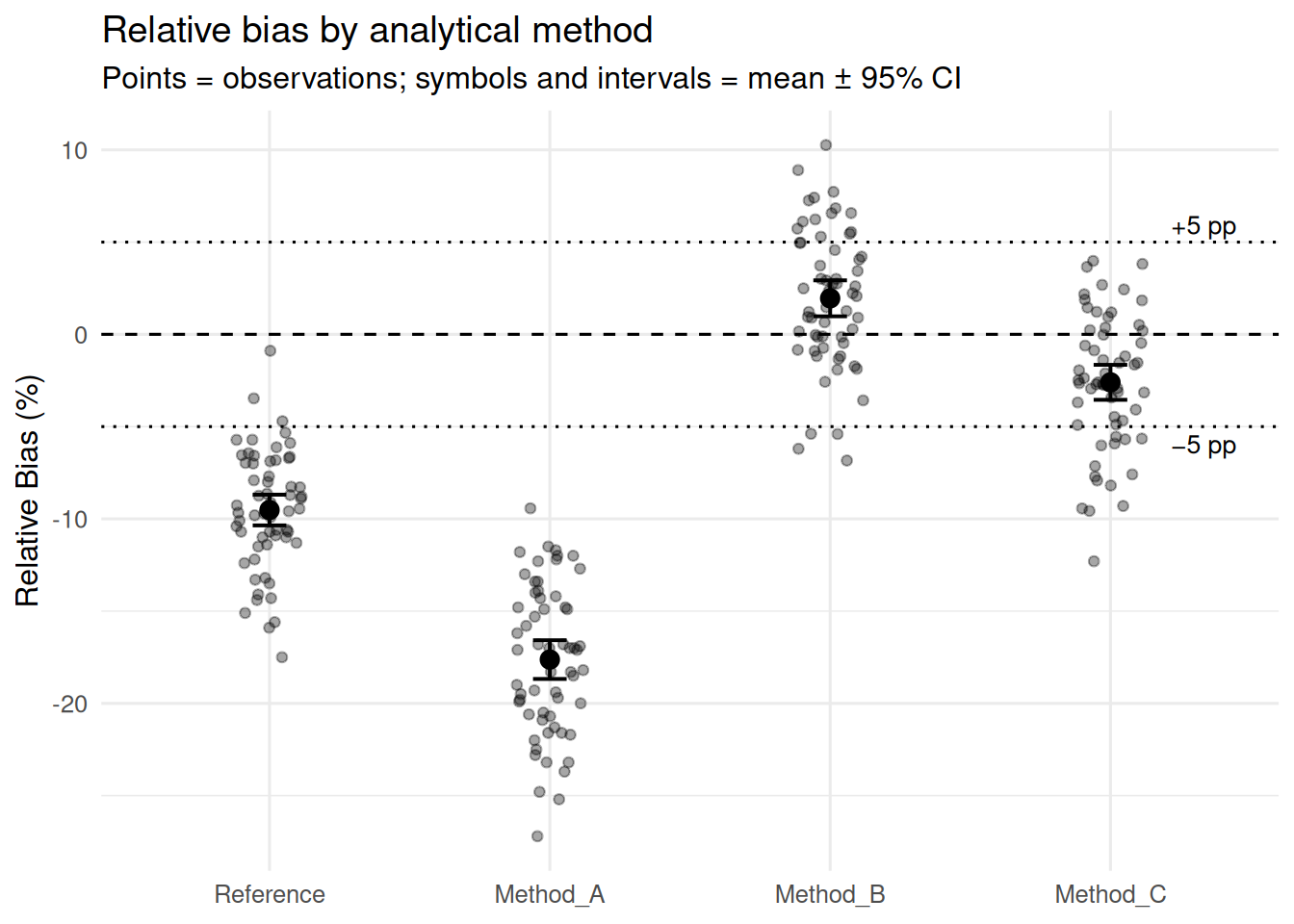
The dotted lines at ±5 percentage points are the predefined chemical relevance threshold.
Visually, the gap between B and C is smaller than the gap between either of them and the other methods.
Whether that gap is statistically distinguishable from zero is a separate question from whether it exceeds the chemical threshold.
Contrast 1: Is the Reference method itself unbiased?
This is not a comparison between two methods.
It is a one-sample question about the Reference method alone:
\[
H_0: \mu_\mathrm{Reference} = 0
\]
ref_bias <- dat[Method =="Reference", RelativeBias_pct]t.test(ref_bias, mu =0)
    One Sample t-test

data:  ref_bias
t = -22.858, df = 59, p-value < 2.2e-16
alternative hypothesis: true mean is not equal to 0
95 percent confidence interval:
 -10.355565  -8.688435
sample estimates:
mean of x
   -9.522
The test gives t = -22.86 with p < 0.001.
The Reference method is significantly biased.
This matters scientifically.
If the Reference method were unbiased, there would be less justification for developing alternatives.
The fact that it is biased — and substantially so — is part of the problem.
Contrast 2: Method B versus Method C
In our scenario, the comparison between B and C is particularly relevant because these are the two strongest candidates.
The question is whether the difference between them is large enough to matter.
We formulate this as a contrast:
\[
C = \mu_B - \mu_C
\]
with coefficients \(0\), \(0\), \(1\), \(-1\).
Because the design is balanced and the group sizes are equal, the standard error of this contrast is:
\[
SE = \sqrt{\frac{s_B^2}{n_B} + \frac{s_C^2}{n_C}}
\]
All six pairwise differences are statistically significant at the 5% level.
But look at the magnitudes, not just the p-values:
Comparison
Difference (pp)
Chemically relevant?
A vs B
-19.6
Yes
A vs C
-15
Yes
A vs Ref
-8.1
Yes
B vs C
-4.6
Borderline
B vs Ref
11.5
Yes
C vs Ref
6.9
Yes
The Tukey table confirms what we already suspected.
Method B and Method C are the two best candidates.
Their difference is real but small.
In a regulatory context, both might be considered “accurate enough”, and the choice could shift to other criteria: precision, cost, throughput, or matrix-specific performance.
Statistical significance versus chemical relevance
This distinction is worth repeating.
The p-value from a contrast tells us whether the observed difference is compatible with a null hypothesis of no difference.
It does not tell us whether the difference matters in the laboratory.
For that, we need a scientific criterion.
In this project, that criterion is:
\[
\boxed{5\text{ percentage points}}
\]
A difference of 4.6 pp between B and C is:
Precisely estimated (small standard error, large sample).
Statistically distinguishable from zero.
Below the threshold that would make us prefer one method over the other on accuracy grounds alone.
This is not a failure of statistics.
It is statistics working as intended.
The data have told us that the difference is real but small.
The decision of whether “small” matters is scientific, not statistical.
What assumptions have we made?
The contrasts we have computed rely on the same assumptions as the one-way ANOVA:
Independence of observations.
Normally distributed residuals.
Common residual variance across methods.
Because this is a classical ANOVA contrast, its standard error is based on the common residual variance estimated by the model. This is one reason why the assumptions of the underlying model matter for contrasts as well as for the global F-test.
If the variances differ substantially between methods, this standard error may not be optimal.
We will investigate this in Chapter 07.
For now, we note the assumption and move on.
What the contrasts tell us — and what they do not
What they tell us
The Reference method is significantly biased.
Method A is substantially worse than all other methods.
Method B and Method C are the best candidates.
Their difference is statistically significant but chemically borderline.
What they do not tell us
Matrix effects: These contrasts average over Fill, Soil and Sediment. If Method B is excellent in one matrix and poor in another, the average is misleading.
Precision: We have looked only at mean bias. A method with zero bias but high variance is still problematic.
Why the differences exist: These comparisons quantify differences between methods under this experimental setup. They do not, by themselves, identify the physical or chemical mechanism responsible for those differences.
Take-home message
A contrast is a question dressed as mathematics.
The coefficients you choose should reflect the scientific questions you actually need to answer.
R’s default output — comparisons against a baseline — is convenient for software.
It is not necessarily the most interesting comparison for your laboratory.
The Tukey HSD gives you all pairwise answers with proper multiplicity adjustment.
But only you can decide which differences are large enough to act on.
And that decision requires both statistical evidence and a scientific threshold.
Next: Two-way ANOVA
We now know which method differences exist and how large they are.
But all of these contrasts average over Matrix.
What if the ranking of methods changes depending on whether the sample is Fill, Soil or Sediment?
That question cannot be answered by one-way ANOVA.
It requires a second factor.
Next, we move to two-way ANOVA.
The question becomes:
Does Matrix influence the bias, and does it do so independently of Method?