library(here)
library(data.table)
library(ggplot2)

dat <- fread(
  here("data", "dataset_v01_clean_balanced.csv")
)

dat[, Method := factor(
  Method,
  levels = c("Reference", "Method_A", "Method_B", "Method_C")
)]

dat[, Matrix := factor(
  Matrix,
  levels = c("Fill", "Soil", "Sediment")
)]04 — Interactions
When the effect of a factor depends on the level of another
Scientific question
The additive model assumed that the effect of Method is the same in every Matrix.
But analytical chemists know that matrix interference rarely behaves so politely.
A method that works well in low-organic Fill may fail in high-organic Sediment.
The real question is therefore:
Does the difference between methods change depending on the matrix?
If it does, we have an interaction.
An interaction does not merely add complexity.
It changes the scientific question.
We can no longer describe method performance adequately with a single average difference across all matrices. Instead, we need to ask how the methods compare within each matrix.
The dataset
We continue with the same balanced dataset.
Two factors are involved:
Method: 4 levelsMatrix: 3 levels
There are 20 observations per Method × Matrix combination, giving 240 observations overall.
Each sample is represented by measurements obtained with all four methods. For the introductory analyses in this series, we continue to treat the analytical observations as independent observations within the linear model. This is a deliberate simplification: the model does not yet explicitly represent the sample-to-sample variation shared by the four method measurements.
That issue will become relevant later when we consider more complex sources of variation.
Load the data
Look at the data: the interaction plot
Before fitting an interaction model, it is useful to look directly at the cell means.
An interaction plot displays the mean response for each combination of Method and Matrix.
If the effect of Method were the same across matrices, the differences between methods would remain approximately constant from one matrix to another. In a standard interaction plot, this corresponds to approximately parallel lines.
Pronounced departures from parallelism suggest that the effect of one factor may depend on the other.
The plot is therefore an excellent exploratory tool for this question.
It is important, however, not to turn the visual rule into a statistical test: lines that look non-parallel do not by themselves establish an interaction, just as apparently parallel lines do not prove that the interaction is absent.
cell_means <- dat[, .(
  Mean = mean(RelativeBias_pct),
  SD   = sd(RelativeBias_pct),
  SE   = sd(RelativeBias_pct) / sqrt(.N),
  N    = .N
), by = .(Method, Matrix)]

cell_means
Method Matrix Mean SD SE N
<fctr> <fctr> <num> <num> <num> <int>
1: Reference Fill -7.44550 1.719187 0.3844220 20
2: Method_A Fill -14.30650 2.371942 0.5303823 20
3: Method_B Fill 3.42045 3.332940 0.7452681 20
4: Method_C Fill -0.80340 2.878025 0.6435459 20
5: Reference Soil -10.77400 2.797611 0.6255648 20
6: Method_A Soil -17.56500 3.198729 0.7152576 20
7: Method_B Soil 2.48005 3.495915 0.7817105 20
8: Method_C Soil -1.35020 2.974563 0.6651325 20
9: Reference Sediment -10.34650 3.826971 0.8557368 20
10: Method_A Sediment -21.01000 3.417124 0.7640922 20
11: Method_B Sediment -0.04235 3.765225 0.8419299 20
12: Method_C Sediment -5.64900 3.154135 0.7052860 20ggplot(cell_means, aes(x = Matrix, y = Mean, colour = Method, group = Method)) +
geom_line(linewidth = 1.2) +
geom_point(size = 3.5) +
geom_hline(yintercept = 0, linetype = "dashed", colour = "grey50") +
labs(
y = "Mean Relative Bias (%)",
title = "Method × Matrix Interaction",
subtitle = "Non-parallel lines indicate interaction"
) +
theme_minimal(base_size = 12)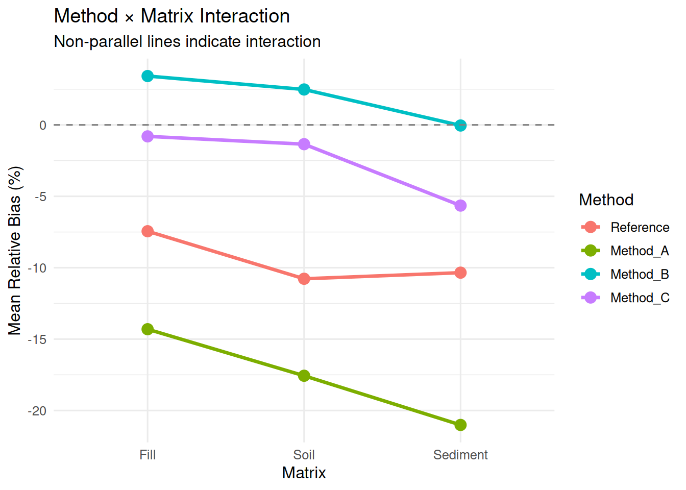
Visually:
- Reference, Method B, Method C: The lines are nearly parallel. The method ranking is stable across matrices.
- Method A: The line drops sharply in Sediment. Method A performs particularly poorly in Sediment compared to Fill and Soil.
The pattern suggests that the difference between methods is not constant across matrices.
But visual inspection is not a statistical test.
We need a model that explicitly represents this possibility.
What is an interaction?
An interaction measures a departure from additivity.
In the additive model, the expected response can be written as:
\[ \mu_{ij} = \mu + \alpha_i + \beta_j \]
where:
\(\mu\) is the overall mean; \(\alpha_i\) represents the effect associated with Method level \(i\); \(\beta_j\) represents the effect associated with Matrix level \(j\).
The important assumption is that the Method effect and the Matrix effect can be added independently.
For example, if moving from Method B to Method A changes the expected bias by the same amount in Fill, Soil and Sediment, the Method effect is additive with Matrix.
An interaction occurs when this additivity is insufficient:
\[ \mu_{ij} \neq \mu + \alpha_i + \beta_j \]
We can therefore extend the model with an interaction term:
\[ \mu + \alpha_i + \beta_j + (\alpha\beta)_{ij} + \varepsilon_{ijk} \]
The interaction term \((\alpha\beta)_{ij}\) represents the part of the Method × Matrix combination that cannot be explained by simply adding the two main effects.
In R formula notation:
Method * Matrix expands to Method + Matrix + Method:Matrix; Method:Matrix represents the interaction terms specifically.
This is the same model written in a different way:
formula_model <- formula(RelativeBias_pct ~ Method * Matrix)

formula_model
RelativeBias_pct ~ Method * MatrixWhat does the model test?
The null hypothesis for the interaction is:
\[ H_0: (\alpha\beta)_{ij} = 0 \quad \text{for all } i, j \]
If we reject this hypothesis, the data provide evidence that method differences vary across matrices.
This does not tell us why the interaction occurs. It only establishes that an additive description is inadequate for the observed data.
And once an interaction is present, the main effects require more careful interpretation.
Fitting the model
fit_int <- lm(RelativeBias_pct ~ Method * Matrix, data = dat)
summary(fit_int)
Call:
lm(formula = RelativeBias_pct ~ Method * Matrix, data = dat)

Residuals:
    Min      1Q  Median      3Q     Max
-8.6801 -2.0998 -0.0172  2.0009  9.4565

Coefficients:
                              Estimate Std. Error t value Pr(>|t|)
(Intercept)                    -7.4455     0.6998 -10.639  < 2e-16 ***
MethodMethod_A                 -6.8610     0.9897  -6.932 4.21e-11 ***
MethodMethod_B                 10.8659     0.9897  10.979  < 2e-16 ***
MethodMethod_C                  6.6421     0.9897   6.711 1.51e-10 ***
MatrixSoil                     -3.3285     0.9897  -3.363 0.000904 ***
MatrixSediment                 -2.9010     0.9897  -2.931 0.003721 **
MethodMethod_A:MatrixSoil       0.0700     1.3997   0.050 0.960158
MethodMethod_B:MatrixSoil       2.3881     1.3997   1.706 0.089341 .
MethodMethod_C:MatrixSoil       2.7817     1.3997   1.987 0.048079 *
MethodMethod_A:MatrixSediment  -3.8025     1.3997  -2.717 0.007100 **
MethodMethod_B:MatrixSediment  -0.5618     1.3997  -0.401 0.688522
MethodMethod_C:MatrixSediment  -1.9446     1.3997  -1.389 0.166097
---
Signif. codes:  0 '***' 0.001 '**' 0.01 '*' 0.05 '.' 0.1 ' ' 1

Residual standard error: 3.13 on 228 degrees of freedom
Multiple R-squared:  0.8634,    Adjusted R-squared:  0.8568
F-statistic:   131 on 11 and 228 DF,  p-value: < 2.2e-16
With the default treatment contrasts used by R, the coefficients are expressed relative to the baseline combination:
Reference + Fill
The model therefore contains:
- the expected mean for Reference in Fill;
- Method effects within Fill;
- Matrix effects within Reference;
- interaction terms describing how those Method effects change when Matrix changes.
This is an important point.
The coefficient labelled Method_A, for example, is not the overall effect of Method A across all matrices. It is the difference between Method A and Reference at the baseline matrix, Fill.
Likewise, a coefficient such as Method_A:Matrix_Sediment describes how the Method A versus Reference difference changes when moving from Fill to Sediment.
Coefficients in an interaction model are therefore conditional on the reference levels used for the other factor.
Changing the factor reference levels changes the individual coefficient values, but not the fitted cell means or the underlying model.
This is one reason why scientific interpretation should usually be based on estimated means, differences, and simple effects rather than on reading individual coefficients in isolation.
The ANOVA table
anova(fit_int)Analysis of Variance Table
Response: RelativeBias_pct
Df Sum Sq Mean Sq F value Pr(>F)
Method 3 13127.4 4375.8 446.7043 < 2.2e-16 ***
Matrix 2 804.8 402.4 41.0777 5.815e-16 ***
Method:Matrix 6 185.9 31.0 3.1624 0.00534 **
Residuals 228 2233.4 9.8
---
Signif. codes: 0 '***' 0.001 '**' 0.01 '*' 0.05 '.' 0.1 ' ' 1The output shows:
- Method: \(F_{3, 228} = 446.7\), \(p < 0.001\)
- Matrix: \(F_{2, 228} = 41.1\), \(p < 0.001\)
- Method:Matrix: \(F_{6, 228} = 3.16\), \(p = 5.3e-03\)
The Method × Matrix interaction is statistically significant.
The evidence therefore argues against the additive assumption that the differences between methods remain constant across matrices.
This is the key result of the episode.
Comparing with the additive model
The interaction model contains the additive model as a special case: setting all interaction terms to zero gives the simpler model.
We can therefore compare the two nested models directly.
fit_add <- lm(RelativeBias_pct ~ Method + Matrix, data = dat)
anova(fit_add, fit_int)
Analysis of Variance Table
Model 1: RelativeBias_pct ~ Method + Matrix
Model 2: RelativeBias_pct ~ Method * Matrix
Res.Df RSS Df Sum of Sq F Pr(>F)
1 234 2419.3
2 228 2233.4 6 185.87 3.1624 0.00534 **
---
Signif. codes: 0 '***' 0.001 '**' 0.01 '*' 0.05 '.' 0.1 ' ' 1The nested F-test asks whether adding the six Method × Matrix interaction parameters produces a sufficiently large reduction in residual variation to justify the additional model complexity.
\(F_{6, 228} = 3.16\), \(p = 5.3e-03\).
The interaction model provides a statistically significant improvement over the additive model.
This does not mean that the additive model was “wrong” from the beginning. It was a simpler model corresponding to a simpler scientific assumption.
The data now give us evidence that this assumption is insufficient.
Simple effects: Method within each Matrix
Once an interaction is present, a single overall Method effect is no longer enough to describe the data.
The scientifically relevant questions become simple effects:
“How do the methods differ within Fill?” “How do the methods differ within Soil?” “How do the methods differ within Sediment?”
One straightforward way to make this idea concrete is to fit the Method comparison separately within each matrix.
for (mx in levels(dat$Matrix)) {
  sub <- dat[Matrix == mx]
  fit_mx <- lm(RelativeBias_pct ~ Method, data = sub)
  cat("\n---", mx, "---\n")
  print(anova(fit_mx))
  cat("R-squared:", summary(fit_mx)$r.squared, "\n")
}
--- Fill ---
Analysis of Variance Table

Response: RelativeBias_pct
          Df Sum Sq Mean Sq F value    Pr(>F)
Method     3 3618.4 1206.13  172.47 < 2.2e-16 ***
Residuals 76  531.5    6.99
---
Signif. codes:  0 '***' 0.001 '**' 0.01 '*' 0.05 '.' 0.1 ' ' 1
R-squared: 0.8719263

--- Soil ---
Analysis of Variance Table

Response: RelativeBias_pct
          Df Sum Sq Mean Sq F value    Pr(>F)
Method     3 4950.0 1649.98  168.68 < 2.2e-16 ***
Residuals 76  743.4    9.78
---
Signif. codes:  0 '***' 0.001 '**' 0.01 '*' 0.05 '.' 0.1 ' ' 1
R-squared: 0.8694219

--- Sediment ---
Analysis of Variance Table

Response: RelativeBias_pct
          Df Sum Sq Mean Sq F value    Pr(>F)
Method     3 4744.9 1581.65  125.41 < 2.2e-16 ***
Residuals 76  958.5   12.61
---
Signif. codes:  0 '***' 0.001 '**' 0.01 '*' 0.05 '.' 0.1 ' ' 1
R-squared: 0.8319422
The estimated cell means make the pattern easier to interpret than the individual F-tests.
method_matrix_means <- dcast(
  cell_means,
  Matrix ~ Method,
  value.var = "Mean"
  )

method_matrix_means
Key: <Matrix>
Matrix Reference Method_A Method_B Method_C
<fctr> <num> <num> <num> <num>
1: Fill -7.4455 -14.3065 3.42045 -0.8034
2: Soil -10.7740 -17.5650 2.48005 -1.3502
3: Sediment -10.3465 -21.0100 -0.04235 -5.6490In all three matrices, Method B and Method C remain the strongest candidates overall, while Method A performs worst.
The important point is not that the ranking changes completely.
It is that the magnitude of the method differences changes with Matrix.
In particular, Method A becomes substantially more negative in Sediment.
This is precisely what the interaction term captures.
A note about inference
The separate models above are useful for understanding the structure of the interaction, but they should not automatically be interpreted as three independent confirmatory tests.
Once we start asking several matrix-specific questions, multiplicity becomes relevant again.
For a formal analysis, simple effects and their contrasts should be defined explicitly and, where appropriate, adjusted for the family of comparisons being made.
Here we use the separate models primarily to make the interaction concrete. More formal contrast-based approaches will become increasingly useful as the models become more complex.
Simple effects: Matrix within each Method
We can also ask the complementary question:
“Does Matrix matter within each method?”
for (m in levels(dat$Method)) {
  sub <- dat[Method == m]
  fit_m <- lm(RelativeBias_pct ~ Matrix, data = sub)
  cat("\n---", m, ": Matrix effect ---\n")
  print(anova(fit_m))
  cat("R-squared:", summary(fit_m)$r.squared, "\n")
}
--- Reference : Matrix effect ---
Analysis of Variance Table

Response: RelativeBias_pct
          Df Sum Sq Mean Sq F value   Pr(>F)
Matrix     2 131.18  65.592  7.7385 0.001063 **
Residuals 57 483.13   8.476
---
Signif. codes:  0 '***' 0.001 '**' 0.01 '*' 0.05 '.' 0.1 ' ' 1
R-squared: 0.2135441

--- Method_A : Matrix effect ---
Analysis of Variance Table

Response: RelativeBias_pct
          Df Sum Sq Mean Sq F value   Pr(>F)
Matrix     2 449.49 224.743  24.486 2.11e-08 ***
Residuals 57 523.16   9.178
---
Signif. codes:  0 '***' 0.001 '**' 0.01 '*' 0.05 '.' 0.1 ' ' 1
R-squared: 0.4621267

--- Method_B : Matrix effect ---
Analysis of Variance Table

Response: RelativeBias_pct
          Df Sum Sq Mean Sq F value   Pr(>F)
Matrix     2 128.25  64.126  5.1292 0.008947 **
Residuals 57 712.63  12.502
---
Signif. codes:  0 '***' 0.001 '**' 0.01 '*' 0.05 '.' 0.1 ' ' 1
R-squared: 0.1525211

--- Method_C : Matrix effect ---
Analysis of Variance Table

Response: RelativeBias_pct
          Df Sum Sq Mean Sq F value    Pr(>F)
Matrix     2 281.72 140.862  15.605 3.936e-06 ***
Residuals 57 514.51   9.027
---
Signif. codes:  0 '***' 0.001 '**' 0.01 '*' 0.05 '.' 0.1 ' ' 1
R-squared: 0.3538189
Method A shows a strong dependence on Matrix:
fit_A_matrix <- lm(
  RelativeBias_pct ~ Matrix,
  data = dat[Method == "Method_A"]
  )

anova(fit_A_matrix)
Analysis of Variance Table
Response: RelativeBias_pct
Df Sum Sq Mean Sq F value Pr(>F)
Matrix 2 449.49 224.743 24.486 2.11e-08 ***
Residuals 57 523.16 9.178
---
Signif. codes: 0 '***' 0.001 '**' 0.01 '*' 0.05 '.' 0.1 ' ' 1The other methods show substantially weaker matrix dependence.
This is consistent with the interaction plot: the methods do not respond to Matrix in the same way.
It is important, however, to distinguish this observation from the formal interaction test.
The interaction asks whether the effects differ across methods. A significant Matrix effect for Method A alone does not, by itself, prove that an interaction exists. The omnibus interaction test provides that formal evidence.
What the interaction tells us chemically
An interaction in analytical chemistry can be a statistical signature of a matrix-dependent analytical effect.
A method that performs adequately in a low-organic Fill may behave differently in a high-organic Sediment if some aspect of the matrix interferes with the analytical procedure.
In our dataset, Method A deteriorates particularly strongly in Sediment, where organic matter is higher.
This suggests a plausible chemical hypothesis:
Could organic matter be one of the variables driving the matrix-dependent behaviour of Method A?
That is a hypothesis, not a conclusion from the interaction model.
The model detects a pattern in the response. It does not identify the chemical mechanism responsible for that pattern.
This distinction matters: statistical association can tell us where to look for an explanation, but not necessarily what the explanation is.
Statistical significance versus chemical relevance
The interaction is statistically significant.
But statistical significance alone does not tell us whether the observed differences matter for the analytical application.
For Method A, the difference between its mean bias in Fill and Sediment is:
mean_A_fill <- cell_means[
  Method == "Method_A" & Matrix == "Fill",
  Mean
]

mean_A_sediment <- cell_means[
  Method == "Method_A" & Matrix == "Sediment",
  Mean
]

difference_A <- abs(mean_A_sediment - mean_A_fill)

cat(
  "Method A: Fill vs Sediment =",
  round(difference_A, 1),
  "percentage points\n"
)
Method A: Fill vs Sediment = 6.7 percentage pointsThis difference is well above our predefined 5 percentage-point threshold for practical relevance.
For Method B:
mean_B_fill <- cell_means[ Method == "Method_B" & Matrix == "Fill", Mean ]

mean_B_sediment <- cell_means[ Method == "Method_B" & Matrix == "Sediment", Mean ]

difference_B <- abs(mean_B_sediment - mean_B_fill)

cat( "Method B: Fill vs Sediment =", round(difference_B, 1), "percentage points\n" )
Method B: Fill vs Sediment = 3.5 percentage pointsThe corresponding change is much smaller and remains below the 5 percentage-point threshold.
The important distinction is therefore:
- the interaction is statistically detectable;
- part of the interaction is also large enough to be practically relevant;
- the practical importance is not necessarily the same for every method.
The F-test tells us that the Method × Matrix pattern is unlikely to be explained by random variation alone. It does not tell us whether every part of that pattern matters scientifically.
What the model does not tell us
- Why does Method A fail in Sediment?
The model detects the pattern but does not explain the mechanism.
Organic matter is one plausible candidate because its concentration is higher in Sediment, but other matrix properties could also contribute.
We need additional information and a different model to investigate that hypothesis.
- Is the interaction important for every analytical application?
Not necessarily.
If a laboratory never analyses Sediment, poor performance of Method A specifically in Sediment may have little practical consequence.
Statistical importance and application-specific importance are separate questions.
- Does the interaction prove causality?
No.
The interaction describes an association between method performance and matrix. The model does not experimentally manipulate the properties of the matrices and therefore cannot establish a causal chemical mechanism.
- Does the interaction mean that main effects are useless?
No.
The main effects still describe average patterns under the model. The problem is that, when the interaction is substantial, an average Method effect may hide important matrix-specific behaviour.
The interaction changes which summaries are most useful for the scientific question.
What assumptions have we made?
The interaction model relies on the same basic linear-model assumptions as the additive model:
- Independence of the model errors.
- Normally distributed residuals, if we want the classical small-sample F-tests to have their exact theoretical properties.
- A common residual variance across the observations represented by the model.
There is also a modelling assumption specific to this analysis:
- the relationship between the response and the two categorical factors is adequately represented by the chosen factorial structure.
The interaction model does not require the raw response to be normally distributed. The normality assumption concerns the errors around the fitted cell means.
Likewise, independence is not something that can be established simply by inspecting a residual plot. It depends primarily on how the observations were generated and on what constitutes an independent experimental or analytical unit.
For this dataset, we deliberately continue with the introductory independent-observation formulation. Later in the series we will examine situations where shared sources of variation, imbalance, or other departures from the model assumptions change the analysis.
With 12 Method × Matrix cells, assessing the residual structure becomes increasingly important.
We will examine these diagnostics explicitly in Chapter 07.
For now, the important point is simply that a significant interaction does not make the model automatically valid. The assumptions supporting the inference still need to be considered.
One-way → two-way → interaction: what have we gained?
We can compare the three models considered so far.
fit_oneway <- lm(
  RelativeBias_pct ~ Method,
  data = dat
  )

model_summary <- data.table(
  Model = c(
    "One-way",
    "Additive two-way",
    "Interaction"
    ),
  R_squared = c(
    summary(fit_oneway)$r.squared,
    summary(fit_add)$r.squared,
    summary(fit_int)$r.squared
    ),
  Interpretation = c(
    "Methods differ",
    "Methods and Matrix both contribute",
    "The Method effect depends on Matrix"
    )
  )

model_summary
Model R_squared Interpretation
<char> <num> <char>
1: One-way 0.8028269 Methods differ
2: Additive two-way 0.8520440 Methods and Matrix both contribute
3: Interaction 0.8634111 The Method effect depends on MatrixEach step adds information.
None of the earlier models was necessarily “wrong”. They answered progressively richer questions.
The one-way model asked:
Do the methods differ on average?
The additive two-way model asked:
Do Method and Matrix both contribute to the response, assuming their effects are additive?
The interaction model asks:
Does the effect of Method depend on Matrix?
This progression is important because it illustrates a general principle of applied modelling:
Start with the simplest model that answers the scientific question, and add complexity when the scientific question or the data require it.
The statistical journey mirrors the scientific journey.
Take-home message
An interaction changes the question.
When there is no important interaction, an overall method comparison can often provide a useful summary.
When an interaction is present, the relevant question becomes:
Which method performs best for this matrix?
The interaction plot is an excellent way to discover this structure, but the formal model is what allows us to test it.
And an interaction often raises the next scientific question:
What measurable property of the samples might explain why the methods respond differently?
In our dataset, organic matter is an obvious candidate.
That takes us from categorical factors to a continuous covariate — and from ANOVA towards ANCOVA.
Next: Unbalanced designs and ANCOVA
Our design is still balanced, and Matrix is still treated as a categorical factor.
Both of these choices will soon be challenged.
First, we will deliberately break the balance of the design and see why the order of terms in an ANOVA table suddenly matters. This will lead to Type I, Type II and Type III sums of squares, and to the question of what each one is actually testing.
At the same time, the dataset contains a variable that we have deliberately ignored so far:
OrganicMatter_pct.
It varies continuously across the samples and may help explain the matrix-dependent behaviour we have just observed.
ANCOVA will allow us to ask whether the apparent Matrix effect remains after accounting for organic matter, and eventually whether different methods have different sensitivities to it.
The dataset has not changed.
Our question has.