10 — Mixed Models

How do we model hierarchical structure?

Scientific question

Throughout this series, we have treated the observations in our dataset as if they were independent.

But the experimental design tells us otherwise.

We have 60 samples, and each sample was analysed with all four methods.

This means that the four measurements obtained from the same sample share something important: they come from the same physical material.

They may therefore be more similar to one another than measurements obtained from different samples.

The question is:

“How should we account for the fact that observations from the same sample are not independent?”

This is the problem addressed by mixed-effects models.

The goal is not to make the model more complicated.

The goal is to make the model reflect the experimental design.

The dataset

We return to the balanced dataset used throughout the previous chapters.

There are:

• 3 matrices;
• 4 analytical methods;
• 60 samples;
• 4 observations per sample;
• 240 observations in total.

The important variable for this chapter is SampleID.

Each SampleID identifies one environmental sample that was analysed using all four methods.

library(here)
library(data.table)
library(ggplot2)
library(lme4)

dat <- fread(
  here("data", "dataset_v01_clean_balanced.csv")
)

dat[, Method := factor(
  Method,
  levels = c("Reference", "Method_A", "Method_B", "Method_C")
)]

dat[, Matrix := factor(
  Matrix,
  levels = c("Fill", "Soil", "Sediment")
)]

dat[, SampleID := factor(SampleID)]

cat("Observations:", nrow(dat), "\n")

Observations: 240 

cat("Samples:", uniqueN(dat$SampleID), "\n")

Samples: 60 

dat[, .N, by = SampleID][, table(N)]

N
 4 
60 

Every sample contributes four observations.

This is not a coincidence in the dataset: it is a consequence of the experimental design.

We therefore have a repeated-measures structure:

\[ \text{Sample} \rightarrow \begin{cases} \text{Reference}\\ \text{Method A}\\ \text{Method B}\\ \text{Method C} \end{cases} \]

The observations are repeated measurements on the same underlying sample.

The problem with treating everything as independent

Consider two measurements:

• Method A applied to FIL_01;
• Method B applied to FIL_01.

They are not independent in the same sense as:

• Method A applied to FIL_01;
• Method B applied to FIL_12.

The first pair shares the same physical sample.

The second pair does not.

The fixed-effects model used earlier was:

fit_fixed <- lm(
  RelativeBias_pct ~ Method * Matrix,
  data = dat
)

summary(fit_fixed)

Call:
lm(formula = RelativeBias_pct ~ Method * Matrix, data = dat)

Residuals:
    Min      1Q  Median      3Q     Max 
-8.6801 -2.0998 -0.0172  2.0009  9.4565 

Coefficients:
                              Estimate Std. Error t value Pr(>|t|)    
(Intercept)                    -7.4455     0.6998 -10.639  < 2e-16 ***
MethodMethod_A                 -6.8610     0.9897  -6.932 4.21e-11 ***
MethodMethod_B                 10.8659     0.9897  10.979  < 2e-16 ***
MethodMethod_C                  6.6421     0.9897   6.711 1.51e-10 ***
MatrixSoil                     -3.3285     0.9897  -3.363 0.000904 ***
MatrixSediment                 -2.9010     0.9897  -2.931 0.003721 ** 
MethodMethod_A:MatrixSoil       0.0700     1.3997   0.050 0.960158    
MethodMethod_B:MatrixSoil       2.3881     1.3997   1.706 0.089341 .  
MethodMethod_C:MatrixSoil       2.7817     1.3997   1.987 0.048079 *  
MethodMethod_A:MatrixSediment  -3.8025     1.3997  -2.717 0.007100 ** 
MethodMethod_B:MatrixSediment  -0.5618     1.3997  -0.401 0.688522    
MethodMethod_C:MatrixSediment  -1.9446     1.3997  -1.389 0.166097    
---
Signif. codes:  0 '***' 0.001 '**' 0.01 '*' 0.05 '.' 0.1 ' ' 1

Residual standard error: 3.13 on 228 degrees of freedom
Multiple R-squared:  0.8634,    Adjusted R-squared:  0.8568 
F-statistic:   131 on 11 and 228 DF,  p-value: < 2.2e-16

This model is perfectly legitimate as a fixed-effects model, but its residual structure assumes independent errors.

In other words, it treats the 240 observations as if they were 240 independent experimental units.

They are not.

This is a form of pseudoreplication.

The problem is not that the model has too few observations.

The problem is that it has less independent information than the number 240 suggests.

What is the experimental unit?

This distinction is fundamental.

The experimental unit is the unit that receives the treatment independently.

Here, the environmental sample is the natural experimental unit for comparing analytical methods.

The four method measurements are therefore repeated observations associated with the same sample.

We should not simply count:

\[ 60 \times 4 = 240 \]

and conclude that we have 240 independent observations.

We have 60 samples measured four times.

That distinction is exactly what the mixed model allows us to represent.

A random intercept for SampleID

The simplest solution is to give each sample its own random intercept.

The model becomes:

\[ Y_{ijk} = \mu + \alpha_i + \beta_j + (\alpha\beta)_{ij} + u_k + \varepsilon_{ijk} \]

where:

• \(\alpha_i\) is the effect of Method;
• \(\beta_j\) is the effect of Matrix;
• \((\alpha\beta)_{ij}\) is the Method × Matrix interaction;
• \(u_k\) is the sample-specific random effect;
• \(\varepsilon_{ijk}\) is the remaining residual error.

We assume:

\[ u_k \sim N(0,\sigma^2_{\text{sample}}) \]

and

\[ \varepsilon_{ijk} \sim N(0,\sigma^2) \]

The important idea is simple:

Each sample is allowed to have its own baseline level of relative bias.

Some samples may tend to produce higher values.

Others may tend to produce lower values.

The mixed model accounts for this shared sample-to-sample variation rather than forcing it into the residual error.

Fitting the mixed model

fit_mixed <- lmer(
  RelativeBias_pct ~ Method * Matrix + (1 | SampleID),
  data = dat
)

summary(fit_mixed)

Linear mixed model fit by REML ['lmerMod']
Formula: RelativeBias_pct ~ Method * Matrix + (1 | SampleID)
   Data: dat

REML criterion at convergence: 1196.2

Scaled residuals: 
     Min       1Q   Median       3Q      Max 
-2.53648 -0.62502 -0.00756  0.57549  2.94172 

Random effects:
 Groups   Name        Variance Std.Dev.
 SampleID (Intercept) 1.522    1.234   
 Residual             8.274    2.876   
Number of obs: 240, groups:  SampleID, 60

Fixed effects:
                              Estimate Std. Error t value
(Intercept)                    -7.4455     0.6998 -10.639
MethodMethod_A                 -6.8610     0.9096  -7.543
MethodMethod_B                 10.8659     0.9096  11.946
MethodMethod_C                  6.6421     0.9096   7.302
MatrixSoil                     -3.3285     0.9897  -3.363
MatrixSediment                 -2.9010     0.9897  -2.931
MethodMethod_A:MatrixSoil       0.0700     1.2864   0.054
MethodMethod_B:MatrixSoil       2.3881     1.2864   1.856
MethodMethod_C:MatrixSoil       2.7817     1.2864   2.162
MethodMethod_A:MatrixSediment  -3.8025     1.2864  -2.956
MethodMethod_B:MatrixSediment  -0.5618     1.2864  -0.437
MethodMethod_C:MatrixSediment  -1.9446     1.2864  -1.512

Correlation of Fixed Effects:
                  (Intr) MthM_A MthM_B MthM_C MtrxSl MtrxSd MthdMthd_A:MtrxSl
MethdMthd_A       -0.650                                                     
MethdMthd_B       -0.650  0.500                                              
MethdMthd_C       -0.650  0.500  0.500                                       
MatrixSoil        -0.707  0.460  0.460  0.460                                
MatrixSdmnt       -0.707  0.460  0.460  0.460  0.500                         
MthdMthd_A:MtrxSl  0.460 -0.707 -0.354 -0.354 -0.650 -0.325                  
MthdMthd_B:MtrxSl  0.460 -0.354 -0.707 -0.354 -0.650 -0.325  0.500           
MthdMthd_C:MtrxSl  0.460 -0.354 -0.354 -0.707 -0.650 -0.325  0.500           
MthdMthd_A:MtrxSd  0.460 -0.707 -0.354 -0.354 -0.325 -0.650  0.500           
MthdMthd_B:MtrxSd  0.460 -0.354 -0.707 -0.354 -0.325 -0.650  0.250           
MthdMthd_C:MtrxSd  0.460 -0.354 -0.354 -0.707 -0.325 -0.650  0.250           
                  MthdMthd_B:MtrxSl MthdMthd_C:MtrxSl MthdMthd_A:MtrxSd
MethdMthd_A                                                            
MethdMthd_B                                                            
MethdMthd_C                                                            
MatrixSoil                                                             
MatrixSdmnt                                                            
MthdMthd_A:MtrxSl                                                      
MthdMthd_B:MtrxSl                                                      
MthdMthd_C:MtrxSl  0.500                                               
MthdMthd_A:MtrxSd  0.250             0.250                             
MthdMthd_B:MtrxSd  0.500             0.250             0.500           
MthdMthd_C:MtrxSd  0.250             0.500             0.500           
                  MthdMthd_B:MtrxSd
MethdMthd_A                        
MethdMthd_B                        
MethdMthd_C                        
MatrixSoil                         
MatrixSdmnt                        
MthdMthd_A:MtrxSl                  
MthdMthd_B:MtrxSl                  
MthdMthd_C:MtrxSl                  
MthdMthd_A:MtrxSd                  
MthdMthd_B:MtrxSd                  
MthdMthd_C:MtrxSd  0.500           

The model contains two kinds of effects.

Fixed effects

Method, Matrix, and their interaction are fixed effects.

These are the effects we want to estimate and interpret.

Random effects

SampleID is a random effect.

We are not interested in estimating a separate scientific effect for FIL_01, FIL_02, and so on.

We are interested in accounting for the variation among samples.

This distinction is the essence of a mixed model:

Fixed effects describe the systematic effects we want to study. Random effects describe sources of variation that induce dependence or represent a broader population of experimental units.

How much variation is associated with the sample?

The random-effects output gives us two variance components:

• variation between samples;
• residual variation within samples.

We can extract them directly.

var_comp <- as.data.table(
  as.data.frame(VarCorr(fit_mixed))
)

var_sample <- var_comp[grp == "SampleID", vcov]
var_resid  <- var_comp[grp == "Residual", vcov]

cat("Between-sample variance:", round(var_sample, 3), "\n")

Between-sample variance: 1.522 

cat("Residual variance:", round(var_resid, 3), "\n")

Residual variance: 8.274 

The two components answer different questions.

The between-sample variance describes how much samples differ from one another after accounting for Method and Matrix.

The residual variance describes the remaining observation-level variation.

This decomposition is one of the main advantages of the mixed model.

The intraclass correlation coefficient

We can summarise the relative importance of the sample effect with the intraclass correlation coefficient, or ICC.

For a random-intercept model:

\[ ICC = \frac{\sigma^2_{\text{sample}}} {\sigma^2_{\text{sample}}+\sigma^2} \]

icc <- var_sample / (var_sample + var_resid)

cat("ICC:", round(icc, 3), "\n")

ICC: 0.155 

cat("Percentage of variance associated with samples:",
    round(100 * icc, 1), "%\n")

Percentage of variance associated with samples: 15.5 %

An ICC of 0.155 means that approximately 15.5% of the modelled variance is associated with differences between samples.

This is not a measure of method performance.

It is a measure of within-sample dependence.

A larger ICC means that measurements from the same sample tend to resemble one another more closely, because they share a common sample-level component.

That is precisely the structure that the random intercept is designed to capture.

In our experimental setup, the four aliquots from the same sample are prepared independently and submitted to the four analytical methods. Independent aliquot preparation can reduce shared preparation errors, but the aliquots still inherit the same underlying sample characteristics.

They are therefore distinct analytical measurements, but they are not four independent samples.

The mixed model explicitly represents this distinction by separating sample-level variation from the remaining observation-level variation.

In our data, approximately 15.5% of the total modelled variance is associated with differences between samples after accounting for Method, Matrix and their interaction.

This suggests that sample-specific heterogeneity remains relevant to the response.

From an analytical-chemistry perspective, this is an important result: the variability between environmental samples is not negligible compared with the remaining measurement-level variability. The model therefore supports treating SampleID as part of the dependence structure rather than treating the 240 measurements as 240 independent experimental units.

Fixed model versus mixed model

It is useful to ask what changes when we acknowledge the sample structure.

The point is not that the mixed model must produce a different scientific conclusion.

The point is that the uncertainty should be estimated under the correct dependence structure.

We can compare the standard error of a method coefficient from the two models.

coef_fixed <- summary(fit_fixed)$coefficients
coef_mixed <- summary(fit_mixed)$coefficients

comparison <- data.table(
  Term = "Method_B",
  SE_fixed = coef_fixed["MethodMethod_B", "Std. Error"],
  SE_mixed = coef_mixed["MethodMethod_B", "Std. Error"]
)

comparison[, Ratio := SE_mixed / SE_fixed]

comparison

       Term  SE_fixed  SE_mixed    Ratio
     <char>     <num>     <num>    <num>
1: Method_B 0.9897353 0.9096152 0.919049

The exact difference is less important than the principle.

The fixed-effects model assumes independent observations.

The mixed model acknowledges that observations from the same sample are correlated.

If the sample effect is important, the two models should not be expected to provide identical uncertainty estimates.

This is why identifying the experimental unit matters before interpreting a p-value.

Testing the fixed effects

The mixed model gives us estimates for the fixed effects, but we still need to ask the same scientific questions as before.

Do methods differ?

Does matrix matter?

Does the method effect depend on matrix?

For this balanced design, we can inspect the fixed-effect coefficients and confidence intervals directly.

confint(fit_mixed, parm = "beta_", method = "Wald")

                                   2.5 %     97.5 %
(Intercept)                   -8.8171779 -6.0738221
MethodMethod_A                -8.6438130 -5.0781870
MethodMethod_B                 9.0831370 12.6487630
MethodMethod_C                 4.8592870  8.4249130
MatrixSoil                    -5.2683455 -1.3886545
MatrixSediment                -4.8408455 -0.9611545
MethodMethod_A:MatrixSoil     -2.4512783  2.5912783
MethodMethod_B:MatrixSoil     -0.1331783  4.9093783
MethodMethod_C:MatrixSoil      0.2604217  5.3029783
MethodMethod_A:MatrixSediment -6.3237783 -1.2812217
MethodMethod_B:MatrixSediment -3.0830783  1.9594783
MethodMethod_C:MatrixSediment -4.4658783  0.5766783

The interpretation of the coefficients remains familiar from the earlier chapters.

What has changed is the error structure.

The Method and Matrix effects are still fixed effects.

The difference is that their uncertainty is now estimated while accounting for the repeated observations within each sample.

Why not add a random slope for Method?

At first glance, we might want to go one step further.

Perhaps the effect of Method is not the same for every sample.

For example, Method A might perform particularly well on some samples and particularly poorly on others.

Conceptually, this suggests a random slope:

lmer(
  RelativeBias_pct ~ Method * Matrix +
    (1 + Method | SampleID),
  data = dat
)

This would allow the Method effect to vary from sample to sample.

However, this model cannot be estimated with our experimental design.

Each sample has exactly four observations:

Reference
Method_A
Method_B
Method_C

A random intercept plus a separate random Method effect therefore attempts to estimate a very large number of sample-specific parameters from only four observations per sample.

With 60 samples and four method-related random coefficients per sample, the random-effects structure contains 240 random effects for 240 observations.

There is no residual information left to identify the model.

lme4 therefore correctly rejects the model.

This is an important lesson:

A more flexible random-effects structure is not automatically a better model.

The data must contain enough repeated information to estimate it.

For this dataset, the random-intercept model is the appropriate level of complexity.

Batch and Day: another layer of the design

The dataset contains additional variables:

• Batch;
• Day;
• Analyst;
• Instrument.

These variables deserve attention, but they do not play the same role as SampleID.

SampleID identifies the physical sample shared by the four method measurements.

Batch and Day describe when and under which analytical conditions a measurement was performed.

This distinction matters.

For example, the four measurements from FIL_01 were not necessarily performed in the same batch or on the same day.

dat[, .(
  n_batch = uniqueN(Batch),
  n_day = uniqueN(Day)
), by = SampleID][, .(
  n_samples = .N
), by = .(n_batch, n_day)][order(n_batch, n_day)]

   n_batch n_day n_samples
     <int> <int>     <int>
1:       2     3         3
2:       2     4         3
3:       3     2         6
4:       3     3        13
5:       3     4        13
6:       4     2         1
7:       4     3         6
8:       4     4        15

The four measurements associated with a sample can therefore span several analytical batches and days.

This means that Batch and Day cannot simply be treated as additional levels of the SampleID hierarchy.

They represent different sources of variation.

Are Batch and Day confounded?

Before adding nuisance variables to a model, it is useful to inspect their structure.

Batch and Day are not perfectly confounded in this dataset.

Several combinations of Batch and Day occur.

with(dat, table(Day, Batch))

        Batch
Day      Batch_01 Batch_02 Batch_03 Batch_04 Batch_05 Batch_06 Batch_07
  Day_01        7        2        1        5        2        2        4
  Day_02        6        4        4        2        7        4        2
  Day_03        3        2        1        2        5        5        0
  Day_04        5        2        2        3        2        2        3
  Day_05        4        0        4        2        2        4        4
  Day_06        4        5        1        9        1        2        1
  Day_07        2        4        1        2        3        3        3
  Day_08        4        2        4        2        1        5        3
  Day_09        1        5        0        4        3        2        5
  Day_10        3        3        2        1        7        2        1
        Batch
Day      Batch_08
  Day_01        3
  Day_02        3
  Day_03        7
  Day_04        1
  Day_05        3
  Day_06        2
  Day_07        2
  Day_08        2
  Day_09        4
  Day_10        3

This is important because complete confounding would make it impossible to distinguish a Batch effect from a Day effect.

Here, the design contains observations across multiple Batch × Day combinations.

That gives us some information with which to separate the two effects.

But this does not mean that both variables must automatically be included in every model.

Model terms should be motivated by the scientific question.

A sensitivity analysis including Batch and Day

We can therefore ask a useful robustness question:

Does the estimated Method effect remain similar after accounting for systematic variation associated with Batch and Day?

For this purpose, we can treat Batch and Day as fixed nuisance effects.

fit_mixed_adj <- lmer(
  RelativeBias_pct ~
    Method * Matrix +
    Batch +
    Day +
    (1 | SampleID),
  data = dat
)

summary(fit_mixed_adj)

Linear mixed model fit by REML ['lmerMod']
Formula: RelativeBias_pct ~ Method * Matrix + Batch + Day + (1 | SampleID)
   Data: dat

REML criterion at convergence: 1165.3

Scaled residuals: 
     Min       1Q   Median       3Q      Max 
-2.39272 -0.67882  0.08215  0.56495  2.57740 

Random effects:
 Groups   Name        Variance Std.Dev.
 SampleID (Intercept) 1.274    1.129   
 Residual             8.597    2.932   
Number of obs: 240, groups:  SampleID, 60

Fixed effects:
                              Estimate Std. Error t value
(Intercept)                   -6.78337    0.99922  -6.789
MethodMethod_A                -7.05597    0.96662  -7.300
MethodMethod_B                10.70042    0.95420  11.214
MethodMethod_C                 6.57469    0.95832   6.861
MatrixSoil                    -3.34659    1.04286  -3.209
MatrixSediment                -2.94995    1.02661  -2.873
BatchBatch_02                  0.21661    0.80249   0.270
BatchBatch_03                 -0.41305    0.87579  -0.472
BatchBatch_04                  0.45061    0.78616   0.573
BatchBatch_05                  0.61447    0.77879   0.789
BatchBatch_06                  0.88937    0.76037   1.170
BatchBatch_07                  1.03871    0.83841   1.239
BatchBatch_08                 -0.39653    0.79123  -0.501
DayDay_02                     -1.25103    0.84457  -1.481
DayDay_03                     -0.86900    0.92509  -0.939
DayDay_04                     -0.87092    0.93481  -0.932
DayDay_05                     -0.50564    0.92563  -0.546
DayDay_06                     -1.56213    0.91304  -1.711
DayDay_07                     -0.34944    0.94844  -0.368
DayDay_08                     -0.84582    0.91270  -0.927
DayDay_09                     -1.76764    0.89894  -1.966
DayDay_10                     -0.78192    0.92459  -0.846
MethodMethod_A:MatrixSoil      0.09919    1.39319   0.071
MethodMethod_B:MatrixSoil      2.62971    1.37486   1.913
MethodMethod_C:MatrixSoil      2.63592    1.34748   1.956
MethodMethod_A:MatrixSediment -3.64132    1.36646  -2.665
MethodMethod_B:MatrixSediment -0.39958    1.35478  -0.295
MethodMethod_C:MatrixSediment -1.76032    1.37008  -1.285

This is not a new scientific hypothesis about Batch or Day.

They are included to control for possible systematic variation associated with analytical runs and measurement days.

The important comparison is therefore between:

Method × Matrix + SampleID

and

Method × Matrix + Batch + Day + SampleID

We can compare the estimated Method coefficients.

get_method_coefs <- function(model) {
  out <- as.data.table(
    coef(summary(model)),
    keep.rownames = "Term"
  )

  out[grepl("^Method", Term),
      .(Term,
        Estimate = Estimate,
        SE = `Std. Error`)]
}

coef_comparison <- merge(
  get_method_coefs(fit_mixed),
  get_method_coefs(fit_mixed_adj),
  by = "Term",
  suffixes = c("_base", "_adjusted")
)

coef_comparison

Key: <Term>
                            Term Estimate_base   SE_base Estimate_adjusted
                          <char>         <num>     <num>             <num>
1:                MethodMethod_A      -6.86100 0.9096152       -7.05597008
2: MethodMethod_A:MatrixSediment      -3.80250 1.2863901       -3.64132013
3:     MethodMethod_A:MatrixSoil       0.07000 1.2863901        0.09918818
4:                MethodMethod_B      10.86595 0.9096152       10.70042441
5: MethodMethod_B:MatrixSediment      -0.56180 1.2863901       -0.39958047
6:     MethodMethod_B:MatrixSoil       2.38810 1.2863901        2.62971093
7:                MethodMethod_C       6.64210 0.9096152        6.57469218
8: MethodMethod_C:MatrixSediment      -1.94460 1.2863901       -1.76031547
9:     MethodMethod_C:MatrixSoil       2.78170 1.2863901        2.63591878
   SE_adjusted
         <num>
1:   0.9666184
2:   1.3664598
3:   1.3931901
4:   0.9542049
5:   1.3547751
6:   1.3748582
7:   0.9583243
8:   1.3700775
9:   1.3474774

If the estimates and their uncertainty remain broadly similar, this provides additional reassurance that the Method conclusions are not simply reflecting differences in Batch or Day.

If they change substantially, that is scientifically important.

It would mean that part of the apparent Method effect is entangled with analytical conditions.

Either outcome is informative.

What about Analyst and Instrument?

The dataset also records the analyst and instrument associated with each measurement.

These are potentially important sources of analytical variation.

However, we should resist the temptation to turn every recorded variable into a random effect.

There are only:

• 3 analysts;
• 2 instruments.

cat("Analysts:", uniqueN(dat$Analyst), "\n")

Analysts: 3 

cat("Instruments:", uniqueN(dat$Instrument), "\n")

Instruments: 2 

cat("Batches:", uniqueN(dat$Batch), "\n")

Batches: 8 

cat("Days:", uniqueN(dat$Day), "\n")

Days: 10 

With only two instruments and three analysts, estimating random-effect variances for these factors would be difficult and would add little to the central lesson of this chapter.

For this dataset, they are better regarded as potential nuisance factors to investigate, rather than automatically adding them to the random-effects structure.

The general principle is:

The presence of a variable in the dataset does not by itself justify including it in the model.

The role of a variable depends on the experimental design and on the scientific question.

Why not make Batch, Day, Analyst and Instrument all random effects?

We could write a model such as:

lmer(
  RelativeBias_pct ~
    Method * Matrix +
    (1 | SampleID) +
    (1 | Batch) +
    (1 | Day) +
    (1 | Analyst) +
    (1 | Instrument),
  data = dat
)

But this would be a poor choice for the main analysis.

There are several reasons.

First, the number of levels is small for Analyst and especially Instrument.

Second, adding random effects does not automatically improve a model.

Third, every additional variance component requires information in the design that can distinguish it from the other sources of variation.

And finally, the central scientific question is still about Method and Matrix.

The purpose of the mixed model is to represent the important dependence structure, not to build the most elaborate model possible.

For this dataset, SampleID is the essential random effect.

Batch and Day are useful as sensitivity adjustments.

Analyst and Instrument should remain part of the design audit unless there is a specific scientific reason to model them.

Diagnostics for the mixed model

A mixed model still has assumptions.

Adding a random effect does not make the model immune to problems with:

• residual normality;
• constant residual variance;
• influential observations;
• misspecification of the fixed-effects structure.

We can inspect the residuals in the same spirit as Chapter 07.

diag_mixed <- data.table(
  fitted = fitted(fit_mixed),
  resid = residuals(fit_mixed),
  std_resid = residuals(fit_mixed, scaled = TRUE)
)

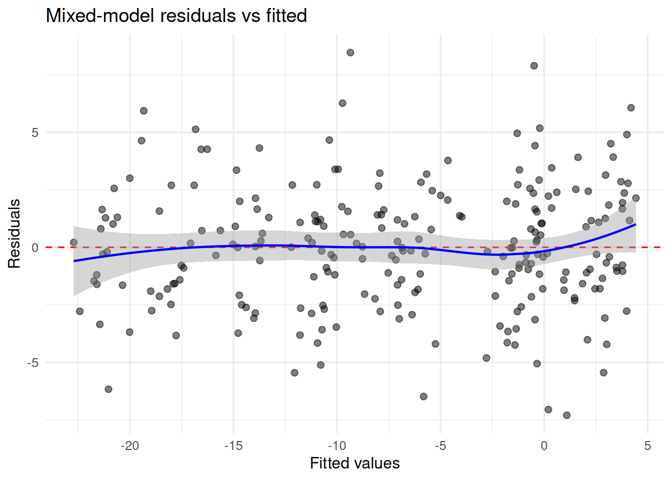
Residuals versus fitted values

ggplot(diag_mixed, aes(x = fitted, y = resid)) +
  geom_point(alpha = 0.5, size = 2) +
  geom_hline(
    yintercept = 0,
    linetype = "dashed",
    colour = "red"
  ) +
  geom_smooth(
    method = "loess",
    se = TRUE,
    colour = "blue",
    linewidth = 0.8
  ) +
  labs(
    x = "Fitted values",
    y = "Residuals",
    title = "Mixed-model residuals vs fitted"
  ) +
  theme_minimal(base_size = 12)

We are looking for the same features as before:

• systematic curvature;
• changing spread;
• isolated extreme observations.

The random effect solves the dependence problem.

It does not solve these other problems automatically.

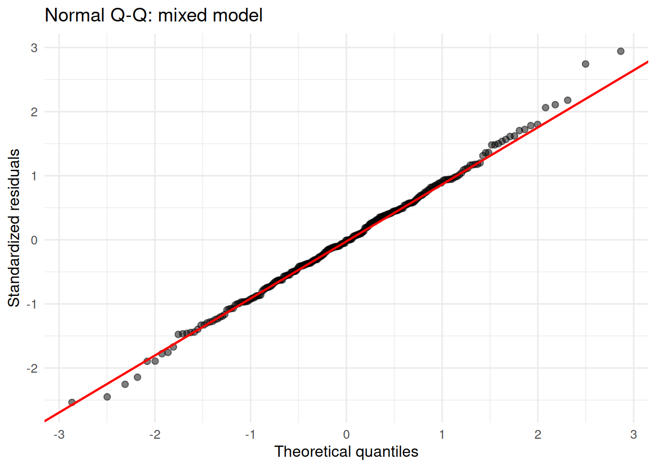
QQ plot of mixed-model residuals

ggplot(diag_mixed, aes(sample = std_resid)) +
  stat_qq(alpha = 0.5, size = 2) +
  stat_qq_line(
    colour = "red",
    linewidth = 0.8
  ) +
  labs(
    x = "Theoretical quantiles",
    y = "Standardized residuals",
    title = "Normal Q-Q: mixed model"
  ) +
  theme_minimal(base_size = 12)

The interpretation is unchanged from Chapter 07.

We are not asking whether the points lie exactly on a mathematical line.

We are asking whether the deviations are large enough to threaten the conclusions we want to draw.

A useful way to think about mixed models

At this point, it is worth stepping back.

The fixed-effects model asks:

How do Method and Matrix affect relative bias?

The mixed model asks:

How do Method and Matrix affect relative bias after accounting for the fact that measurements from the same sample are correlated?

The scientific question has not changed.

The model has changed because our understanding of the experimental design has improved.

This is one of the most important ideas in applied statistics:

The statistical model should follow the data-generating process, not the other way around.

What the mixed model changes — and what it does not

The mixed model does not automatically change:

• the definition of Method;
• the definition of Matrix;
• the interaction between them;
• the scientific interpretation of the response.

It changes the way uncertainty is partitioned.

Part of the variation is now explicitly attributed to differences between samples.

The remaining variation belongs to the observation-level residual.

This can change standard errors and therefore inference.

That is not a defect of the mixed model.

It is the consequence of using a more realistic description of the data.

Take-home message

The important question is not “Do I have a mixed-effects dataset?”

The important question is “Which observations are actually independent?”

Our dataset contains 240 measurements, but only 60 independent samples.

Each sample was analysed by all four methods.

The four observations associated with the same sample therefore share a common source of variation.

A random intercept for SampleID captures this dependence:

RelativeBias_pct ~ Method * Matrix + (1 | SampleID)

The ICC tells us how important the sample-level variation is.

Batch and Day represent additional analytical structure. They are useful for sensitivity analysis and can be included as fixed nuisance effects when we want to ask whether the Method conclusions are robust to these sources of systematic variation.

Analyst and Instrument are also relevant variables, but with only 3 and 2 levels respectively, they do not need to become random effects in our main model.

Finally, a more complicated random-effects structure is not necessarily better.

Our attempt to give each sample a random Method effect fails because four observations per sample do not contain enough information to estimate that structure.

The lesson is simple:

Mixed models are not about adding random effects until the model looks sophisticated.

They are about representing the dependence that is actually present in the experiment.

---

Final reflection

This brings us to an important point in the progression of the series.

We began by treating the dataset as a collection of observations.

Then we asked increasingly specific questions about:

• methods;
• matrices;
• interactions;
• unbalanced designs;
• covariates;
• assumptions;
• robustness.

Now we have asked a more fundamental question:

What exactly is an observation?

A measurement made on a sample is not necessarily an independent experimental unit.

Once we recognise that, the statistical model changes.

This is not a technical refinement added at the end of the analysis.

It is part of understanding the experiment itself.

And that is ultimately what applied statistics requires: not simply fitting models to data, but identifying the structure that generated those data.

---

The complete journey

Chapter	Question
01	Do the four methods have the same mean bias?
02	Which comparisons actually matter?
03	Does Matrix matter independently of Method?
04	Does the method effect depend on the matrix?
05	What happens when the design is unbalanced?
06	Does organic matter explain the pattern?
07	Are the model assumptions defensible?
08	Which conclusions are robust?
09	How repeated measurements should be handled?
10	How does hierarchical structure affect inference?

The statistical journey does not end with the most complicated model.

It ends when the model is appropriate for the question and the structure of the data.