library(here)
library(data.table)
library(ggplot2)
library(car)
library(emmeans)

dat <- fread(
  here("data", "dataset_v01_clean_balanced.csv")
)

dat[, Method := factor(
  Method,
  levels = c("Reference", "Method_A", "Method_B", "Method_C")
)]

dat[, Matrix := factor(
  Matrix,
  levels = c("Fill", "Soil", "Sediment")
)]06 — ANCOVA
Does organic matter explain the pattern we have observed?
Scientific question
We have established that Method and Matrix both influence relative bias, and that they interact.
But we have not yet asked why.
Organic matter content varies systematically across matrices:
- Fill has low organic matter.
- Soil has moderate organic matter.
- Sediment has high organic matter.
And organic matter is known to interfere with many analytical extractions.
The natural question is therefore:
Does organic matter content account for part of the method and matrix differences we have observed?
If it does, the apparent matrix effect may actually be driven primarily by organic matter content.
And if different methods are differentially sensitive to organic matter, that would explain the interaction.
This is the domain of ANCOVA (Analysis of Covariance).
The dataset
We return to the balanced dataset.
- Response:
RelativeBias_pct(continuous) - Primary Factor:
Method(categorical, 4 levels) - Secondary Factor:
Matrix(categorical, 3 levels) - Covariate:
OrganicMatter_pct(continuous)
Load the data
Is organic matter just a proxy for Matrix?
Before fitting models with both a covariate and categorical factors, we must inspect how OrganicMatter_pct relates to Matrix.
If the ranges of organic matter were completely separated by matrix (e.g., Fill = 0-2%, Soil = 5-7%, Sediment = 12-15%), Matrix and OrganicMatter_pct would be fully confounded. In that scenario, including both in a model would cause severe collinearity, making it impossible to separate their effects.
In our dataset, the overlap was designed to be partial:
ggplot(dat, aes(x = Matrix, y = OrganicMatter_pct, fill = Matrix)) +
  geom_boxplot(alpha = 0.6, show.legend = FALSE) +
  geom_jitter(width = 0.15, alpha = 0.4, show.legend = FALSE) +
  labs(
    x = "Environmental Matrix",
    y = "Organic Matter (%)",
    title = "Organic Matter Content by Matrix",
    subtitle = "Partial overlap allows evaluating both terms in the same model"
  ) +
  theme_minimal(base_size = 12)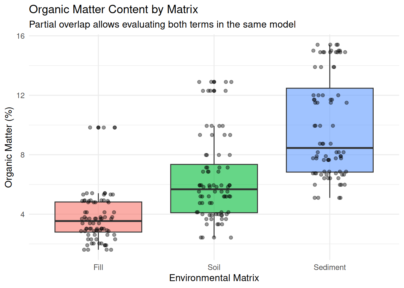
The partial overlap is key:
- Sediment has the highest average organic matter, but its lower range overlaps with Soil.
- Soil overlaps partially with both Fill and Sediment.
This structure allows us to ask two distinct questions:
- Across the entire dataset, does organic matter explain the observed relative bias?
- Controlling for matrix, does organic matter still exert a residual effect, or does
Matrixcarry additional unmeasured complexity?
Look at the data: organic matter and bias
We examine the relationship between organic matter and relative bias across methods.
ggplot(dat, aes(x = OrganicMatter_pct, y = RelativeBias_pct, colour = Method)) +
  geom_point(alpha = 0.5, size = 2) +
  geom_smooth(method = "lm", se = FALSE, linewidth = 1) +
  geom_hline(yintercept = 0, linetype = "dashed", colour = "grey50") +
  labs(
    x = "Organic Matter (%)",
    y = "Relative Bias (%)",
    title = "Relative Bias vs Organic Matter",
    subtitle = "One regression line per method"
  ) +
  theme_minimal(base_size = 12)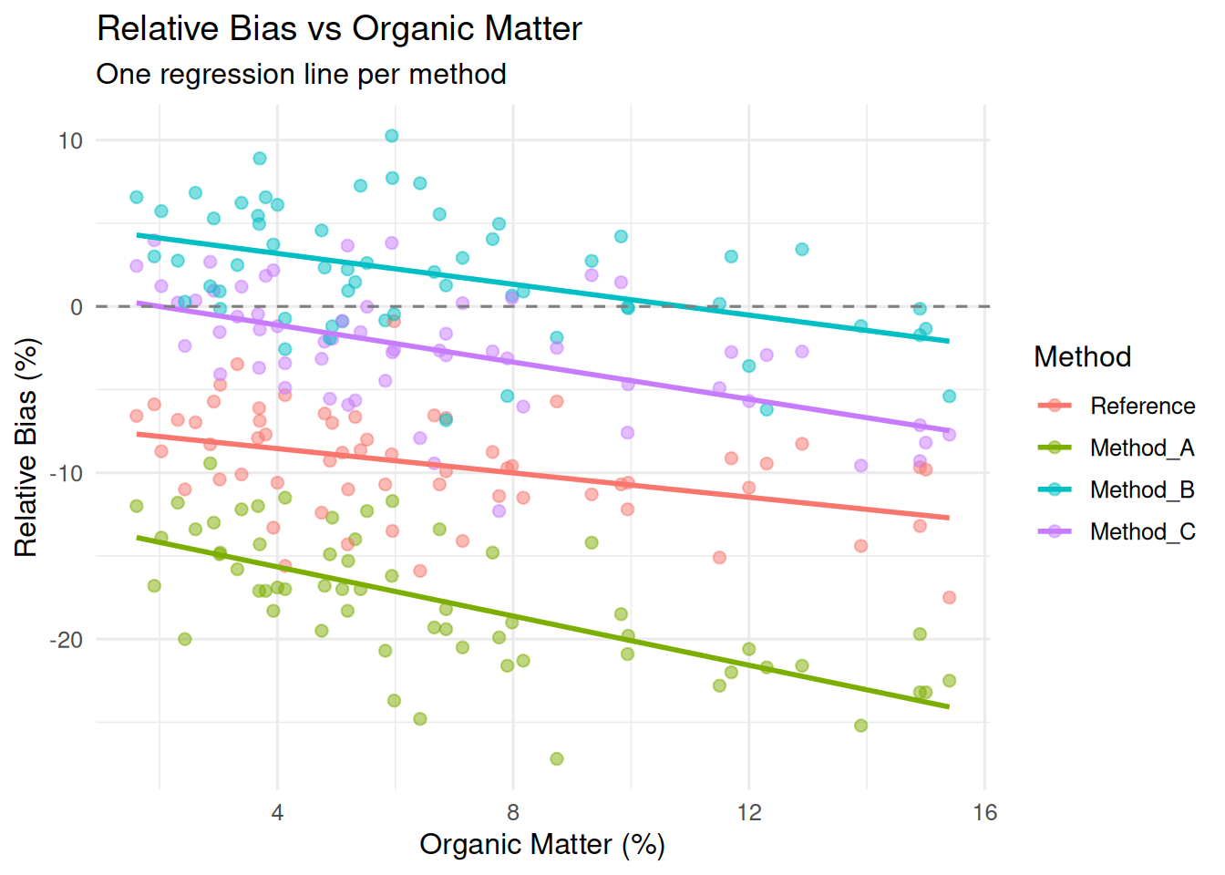
The plot reveals three clear patterns:
- The fitted slopes are generally negative, although the estimated slopes for Reference and Method B are close to zero.
- Method A and Method C show the clearest negative trends.
- The slopes appear to differ: Method A looks steeper than Method B.
- Covariate values vary continuously: organic matter provides a numeric scale within and across matrices.
Model comparison: Additive structures
We compare three additive formulations to see how organic matter interacts with the existing factor structure:
- Two-Way ANOVA:
Method+Matrix - Simple ANCOVA:
Method+OrganicMatter_pct - Combined Additive ANCOVA:
Method+Matrix+OrganicMatter_pct
\[Y_{ijk} = \mu + \text{Method}_i + \text{Matrix}_j + \beta \, X_{ijk} + \varepsilon_{ijk}\]
fit_twoway   <- lm(RelativeBias_pct ~ Method + Matrix, data = dat)
fit_ancova   <- lm(RelativeBias_pct ~ Method + OrganicMatter_pct, data = dat)
fit_full_add <- lm(RelativeBias_pct ~ Method + Matrix + OrganicMatter_pct, data = dat)
Evaluating the combined model using Type II ANOVA (unconditional tests):
car::Anova(fit_full_add, type = "II")Anova Table (Type II tests)
Response: RelativeBias_pct
Sum Sq Df F value Pr(>F)
Method 13127.4 3 467.4009 < 2.2e-16 ***
Matrix 115.2 2 6.1517 0.002492 **
OrganicMatter_pct 238.0 1 25.4172 9.276e-07 ***
Residuals 2181.3 233
---
Signif. codes: 0 '***' 0.001 '**' 0.01 '*' 0.05 '.' 0.1 ' ' 1The output reveals two critical findings:
- Organic matter remains highly significant (\(p < 0.001\)) after controlling for
Matrix. It is a genuine continuous driver of bias, not just an artifact of matrix grouping. Matrixremains significant (\(p < 0.001\)) after adjusting for Organic Matter. Organic matter explains part of the matrix effect, but not all of it. Other matrix properties (e.g., mineralogy, grain size) still contribute to bias.
Adjusted means (emmeans)
In an additive ANCOVA model, emmeans can be used to compare methods at a common value of the covariate, typically its mean. This makes the comparison conditional on the same covariate value rather than on the covariate distributions observed in each group, ensuring a fairer comparison when methods or matrices are evaluated across varying covariate levels.
emm_method <- emmeans::emmeans(fit_full_add, ~ Method)
print(emm_method)
Method emmean SE df lower.CL upper.CL
Reference -9.52 0.395 233 -10.30 -8.74
Method_A -17.63 0.395 233 -18.41 -16.85
Method_B 1.95 0.395 233 1.17 2.73
Method_C -2.60 0.395 233 -3.38 -1.82
Results are averaged over the levels of: Matrix
Confidence level used: 0.95 Comparing raw sample means with adjusted means:
raw_means <- dat[, .(Raw = mean(RelativeBias_pct)), by = Method]
adj_means <- as.data.frame(emm_method)[, c("Method", "emmean")]
setnames(adj_means, "emmean", "Adjusted")

merge(raw_means, adj_means, by = "Method")
Key: <Method>
Method Raw Adjusted
<fctr> <num> <num>
1: Reference -9.522000 -9.522000
2: Method_A -17.627167 -17.627167
3: Method_B 1.952717 1.952717
4: Method_C -2.600867 -2.600867Because our experimental design is perfectly balanced—each method was evaluated on the exact same proportion of Fill, Soil, and Sediment samples—the mean organic matter content within each method group is identical to the overall dataset mean (\(\bar{X}_{i} = \bar{X}_{global}\)).
As a result, the adjustment term \(\hat{\beta}(\bar{X}_{i} - \bar{X}_{global})\) equals zero, making the raw means and adjusted means numerically identical.
This identity is not a coincidence, but a mathematical demonstration of the benefits of orthogonal experimental design:
- No method–covariate imbalance: Because every method was applied to the same samples, the distribution of organic matter is the same across methods.
- Variance Reduction vs. Mean Adjustment: While the covariate adjustment does not alter the point estimates of the method means in a balanced design, it can explain systematic variation that would otherwise remain in the residuals, substantially reducing the residual error variance (\(SS_{residuals}\)), increasing statistical power and tightening confidence intervals.
print(
  c(
    RSS_twoway = deviance(fit_twoway),
    RSS_ancova = deviance(fit_full_add)
    )
)
RSS_twoway RSS_ancova
2419.302 2181.346 In observational studies or unbalanced datasets, \(\bar{X}_{i} \neq \bar{X}_{global}\), and raw means can be deeply misleading. Showing their identity here highlights how ANCOVA protects against confounding when balance is lost.
Testing the interaction: do slopes differ by method?
The visual plot suggested that Method A had a steeper negative slope than the other methods.We test whether the effect of organic matter depends on the method by adding an interaction term:
\[Y_{ijk} = \mu + \text{Method}_i + \text{Matrix}_j + \beta_i \, X_{ijk} + \varepsilon_{ijk}\] This model allows the OM slope to differ between methods, but assumes that the slope is common across matrices. That is another modelling assumption, not a property of ANCOVA itself.
fit_ancova_int <- lm(RelativeBias_pct ~ Method * OrganicMatter_pct + Matrix, data = dat)
car::Anova(fit_ancova_int, type = "II")
Anova Table (Type II tests)
Response: RelativeBias_pct
Sum Sq Df F value Pr(>F)
Method 13127.4 3 474.9655 < 2.2e-16 ***
OrganicMatter_pct 238.0 1 25.8286 7.723e-07 ***
Matrix 115.2 2 6.2513 0.002272 **
Method:OrganicMatter_pct 62.4 3 2.2570 0.082549 .
Residuals 2119.0 230
---
Signif. codes: 0 '***' 0.001 '**' 0.01 '*' 0.05 '.' 0.1 ' ' 1Comparing the interaction model against the additive model:
anova(fit_full_add, fit_ancova_int)Analysis of Variance Table
Model 1: RelativeBias_pct ~ Method + Matrix + OrganicMatter_pct
Model 2: RelativeBias_pct ~ Method * OrganicMatter_pct + Matrix
Res.Df RSS Df Sum of Sq F Pr(>F)
1 233 2181.3
2 230 2119.0 3 62.38 2.257 0.08255 .
---
Signif. codes: 0 '***' 0.001 '**' 0.01 '*' 0.05 '.' 0.1 ' ' 1The interaction test yields \(p > 0.05\). The interaction is not statistically significant.
This is a key pedagogical moment:
- Visually, the slope for Method A appears steeper.
- Incentively, we expect chemical methods to respond differently to matrix interference.
- Statistically, the dataset does not provide sufficient evidence to reject the common slope assumption.
Visual inspection generates hypotheses; formal inference tests whether sampling variability alone could explain the observed pattern.
Centering the covariate and interpreting coefficients
In models with interactions or complex additive structures, centering continuous covariates around their mean (\(\text{OM\_centered} = X - \bar{X}\)) improves coefficient interpretability:
dat[, OM_centered := OrganicMatter_pct - mean(OrganicMatter_pct)]

fit_centered <- lm(RelativeBias_pct ~ Method * OM_centered + Matrix, data = dat)
summary(fit_centered)
Call:
lm(formula = RelativeBias_pct ~ Method * OM_centered + Matrix,
    data = dat)

Residuals:
   Min     1Q Median     3Q    Max
-8.121 -1.682  0.162  1.761  9.649

Coefficients:
                           Estimate Std. Error t value Pr(>|t|)
(Intercept)                -8.39164    0.52136 -16.096  < 2e-16 ***
MethodMethod_A             -8.10517    0.55416 -14.626  < 2e-16 ***
MethodMethod_B             11.47472    0.55416  20.706  < 2e-16 ***
MethodMethod_C              6.92113    0.55416  12.489  < 2e-16 ***
OM_centered                -0.19711    0.11622  -1.696 0.091241 .
MatrixSoil                 -1.10918    0.51219  -2.166 0.031374 *
MatrixSediment             -2.28191    0.64582  -3.533 0.000496 ***
MethodMethod_A:OM_centered -0.37347    0.14975  -2.494 0.013334 *
MethodMethod_B:OM_centered -0.09781    0.14975  -0.653 0.514286
MethodMethod_C:OM_centered -0.19179    0.14975  -1.281 0.201563
---
Signif. codes:  0 '***' 0.001 '**' 0.01 '*' 0.05 '.' 0.1 ' ' 1

Residual standard error: 3.035 on 230 degrees of freedom
Multiple R-squared:  0.8704,    Adjusted R-squared:  0.8653
F-statistic: 171.6 on 9 and 230 DF,  p-value: < 2.2e-16
Centering does not alter model predictions, residual variance, or overall \(p\)-values. However, it changes the meaning of lower-order parameters:
- Intercept (\(-8.39\%\)): Expected bias for the Reference method in Fill matrix at average organic matter content.
- OM_centered (\(-0.197\)): The slope of organic matter for the Reference method. For each additional \(1\%\) of organic matter, relative bias drops by \(\approx 0.2\) percentage points.
- Method_A:OM_centered (\(-0.373\)): The difference in slope between Method A and Reference. The effective slope for Method A is \((-0.197) + (-0.373) = -0.570\), confirming its steeper degradation.
A subtle statistical pitfall: Global test vs Single coefficients
An important nuance emerges when comparing the ANOVA table with the summary table because these two approaches answer fundamentally different questions:
- Global interaction test (\(F = 2.257, p = 0.083\)):
- Question: Are all method-specific slopes compatible with a common slope?
- Interpretation: This omnibus test acts as a safeguard against false discoveries. Because the overall interaction term fails to reach significance at \(\alpha = 0.05\), we cannot formally reject the common slope assumption across the board.
- Method A interaction coefficient (\(t = -2.494, p = 0.013\)):
- Question: Is the slope for Method A different from the slope for the Reference method?
- Interpretation: This specific \(t\)-test focuses entirely on a single contrast. It explains why Method A stood out visually, flagging it as a strong candidate for further study—even if the overall model currently lacks the global evidence to discard a universal slope.
The global test protects against Type I error inflation due to multiple comparisons, while the coefficient test provides localized sensitivity. Rather than treating them as contradictory, view them as complementary: the global test says “proceed with caution regarding the whole interaction structure,” while the specific coefficient points directly to where the action might be happening.
Chemical interpretation
The ANCOVA workflow provides clear answers to our original scientific questions:
- Does organic matter drive bias? Yes. Increasing organic matter content systematically increases negative relative bias across all methods.
- Does organic matter fully explain the Matrix effect? No. Both
OrganicMatter_pctandMatrixremain statistically significant when included together. Organic matter accounts for a major portion of performance degradation, but unmeasured matrix properties still matter. - Do methods differ in their sensitivity to organic matter? Not detectably in this dataset. We cannot claim that Method A is definitively more sensitive to organic matter than Method B, as the interaction term remains non-significant.
Take-home message
ANCOVA is not simply “ANOVA with a covariate tacked on” — it is a tool to disentangle continuous physical drivers from categorical groupings.
Key takeaways from this analysis:
- Verify covariate overlap: If a continuous covariate and a categorical factor do not share overlapping ranges, adjusting for the covariate requires extrapolation and yields unreliable conclusions.
- Continuous drivers reduce error variance: Incorporating organic matter accounts for residual variation, sharpening our estimates of method differences.
- Covariates do not always eliminate factor effects: Organic matter explains part of the matrix effect, but the categorical factor
Matrixretains residual explanatory power. - Distinguish visual trends from statistical evidence: A visual difference in slopes does not guarantee a significant interaction.
Next: Diagnostics
Throughout this series, we have fitted one-way ANOVA, two-way ANOVA, interaction models, and ANCOVA models.
Every one of these models relies on core mathematical assumptions:
- Normality of residuals
- Homoscedasticity (equal variance)
- Independence of observations
- Linearity
Are these assumptions defensible for our analytical data? And what steps should we take if they break down?
Next, we turn to model diagnostics.
The key question becomes:
“Are our model assumptions defensible, and how do we detect and handle their violation?”