But if two measurements come from the same sample, this may not be realistic.
Suppose Sample 17 has unusually high organic matter, an unusual mineral composition, or some other characteristic that makes its relative bias systematically different from the other samples.
That characteristic affects all four method measurements.
The residuals are therefore not simply four unrelated errors.
They share information about the same underlying sample.
The issue is not that we have “too many observations”.
We have 240 measurements.
The issue is that 240 measurements do not contain the same amount of independent information as 240 measurements from unrelated samples.
Look at the data by SampleID
The first step is to make the repeated structure visible.
Every sample contributes exactly four observations.
This is the defining structure of the dataset for the next two chapters.
Visualising within-sample dependence
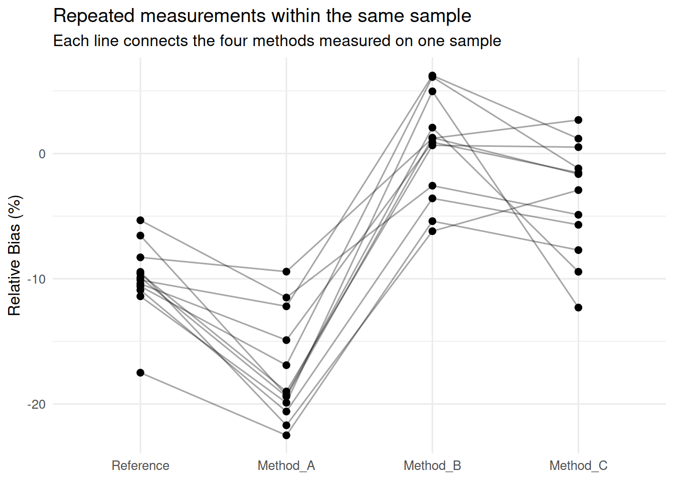
A useful way to see the structure is to connect measurements belonging to the same sample.
We do not need to display all 60 samples.
A random subset is easier to read.
set.seed(42)sample_plot <- dat[ SampleID %in%sample(unique(SampleID), 12)]ggplot( sample_plot,aes(x = Method, y = RelativeBias_pct, group = SampleID)) +geom_line(alpha =0.35) +geom_point(size =2) +labs(x =NULL,y ="Relative Bias (%)",title ="Repeated measurements within the same sample",subtitle ="Each line connects the four methods measured on one sample" ) +theme_minimal(base_size =12)
The lines are not random noise: some samples tend to have relatively high bias across several methods, others tend to have relatively low bias.
The method effect is superimposed on this sample-to-sample variation.
This is exactly the structure that an independent-observations model fails to represent explicitly.
Paired comparisons
There is a simpler statistical idea that already captures part of this structure.
Suppose we wanted to compare Method B with Method C only.
Because both methods were applied to the same 60 samples, we could calculate:
\[
D_k = Y_{k,B} - Y_{k,C}
\]
for each sample \(k\).
The comparison is then based on 60 within-sample differences rather than treating the two methods as unrelated groups.
    Paired t-test

data:  wide_bc$Method_B and wide_bc$Method_C
t = 8.7003, df = 59, p-value = 3.62e-12
alternative hypothesis: true mean difference is not equal to 0
95 percent confidence interval:
 3.506292 5.600875
sample estimates:
mean difference
       4.553583
The paired analysis asks a very specific question:
Within the same sample, is the expected bias different between Method B and Method C?
This is often more informative than an independent-samples comparison because sample-specific variation is removed from the comparison.
The general principle is important:
When measurements are naturally paired, the analysis should respect the pairing.
But a paired t-test is not enough for our full factorial design.
We have four methods, three matrices, and an interaction.
We need a model that can represent all of these structures simultaneously.
Repeated measures as a blocking structure
There is another way to describe the same design.
Each sample can be regarded as a block.
Within a block, all four methods are compared on the same material.
This has a major experimental advantage.
Suppose Sample 17 has unusually high organic matter.
Because all four methods are applied to Sample 17, that unusual characteristic affects all methods within the block.
The comparison between methods can therefore be made while holding the sample itself approximately constant.
This is the logic of a randomized block design: the sample acts as a blocking factor, the method is the treatment we want to compare.
Fixed-effect blocking
One possible model is to include SampleID as a fixed effect:
This model removes systematic differences between samples from the residual error.
It is therefore much closer to the actual experimental comparison than a model that treats SampleID as irrelevant.
But it also introduces 59 additional parameters.
That is not necessarily wrong.
It is simply not the most natural way to describe a population of samples.
We usually do not want to estimate a separate scientific parameter for Sample 1, Sample 2, Sample 3, and so on.
We want to describe how much samples vary from one another.
That is the motivation for random effects.
Fixed effects versus random effects
The distinction is conceptual.
A fixed effect is usually used when the levels themselves are the scientific objects of interest.
For example:
Method A, B and C;
Fill, Soil and Sediment.
We want to compare these specific levels.
A random effect is used when the observed levels represent a sample from a broader population of possible levels, and our interest is primarily in the variability they introduce.
The 60 SampleIDs are a natural example.
We are not interested in whether Sample 17 is different from Sample 23.
We are interested in the fact that samples differ.
That is a variance question.
What about Batch and Day?
The same reasoning can apply to laboratory process variables.
Our dataset contains variables such as:
Batch
Day
Analyst
Instrument
But their presence in the dataset does not automatically mean that they should all become random effects.
The first question is:
Do observations sharing the same level of this variable plausibly share a source of dependence or common variation?
For example, measurements performed in the same analytical batch may share:
reagent preparation;
calibration;
environmental conditions;
instrument state.
Measurements performed on the same day may also share common conditions.
These are plausible sources of clustering.
But there is another question:
Does the experimental design provide enough independent levels to estimate that variance component?
A random effect with only two or three levels is difficult to estimate reliably.
And if Day, Batch, Analyst and Instrument are strongly nested or confounded, adding all of them to the model may create an apparently sophisticated model that the design cannot actually support.
Therefore we will not add them simply because they are available.
They are candidates for random effects only if their experimental structure justifies them.
We will return to this issue in the next chapter.
Why not stop with the paired t-test?
The paired t-test is useful when the scientific question is a single comparison between two methods.
Our question is broader.
We want to estimate:
the effect of Method;
the effect of Matrix;
the Method × Matrix interaction;
while accounting for the fact that observations from the same sample are correlated.
This is more naturally expressed as a hierarchical model.
The structure is:
\[
\text{measurement}
\rightarrow
\text{sample}
\rightarrow
\text{population of samples}
\]
The mixed model provides a way to represent that hierarchy directly.
A useful distinction: dependence versus pseudoreplication
The word pseudoreplication is often used whenever repeated observations are analysed as if they were independent.
But the more precise issue in our dataset is first of all dependence.
The four measurements from a sample are not automatically invalid observations.
They are useful repeated measurements.
The problem arises when the analysis treats them as if they came from independent experimental units.
Whether this constitutes pseudoreplication depends on the experimental question and on what was independently randomized.
The practical lesson is simpler:
Before choosing a statistical test, identify the unit that was independently replicated or randomized.
A diagnostic plot cannot recover this information.
It comes from the experimental design.
What happens to our scientific question?
Earlier we asked:
“Do methods differ?”
Then we asked:
“Does the method effect depend on matrix?”
Now the question becomes:
“Do methods differ within samples, while accounting for the fact that samples themselves vary?”
This is a more precise statement of the experimental comparison.
The statistical model should reflect it.
Take-home message
Repeated measurements are not automatically independent observations.
Our dataset contains 240 measurements, but they are organised into 60 samples with four measurements per sample.
That structure creates dependence.
A paired analysis can account for this when comparing two methods.
A blocked fixed-effects model can account for it by treating SampleID as a fixed blocking factor.
But when the scientific interest is in a population of samples rather than in the 60 observed samples individually, a random-effects formulation is more natural.
This leads directly to mixed-effects models.
The important lesson is not:
“Use a mixed model whenever you have repeated measurements.”
It is:
Identify the dependence structure created by the experimental design, then choose a model that represents the structure relevant to the scientific question.
Next: Mixed Models
We now know why SampleID matters.
The next question is how to represent sample-to-sample variation without estimating a separate fixed effect for every sample.
We will introduce a random intercept for SampleID.
Then we will ask:
“How much of the total variability comes from differences between samples, and how does acknowledging that structure change our inference about Method and Matrix?”