We have developed three alternative analytical methods — A, B and C — and want to compare them with the currently used Reference method.
The scientific question is deliberately simple:
Do the four methods have the same mean relative bias?
If they do not, we will eventually want to know which methods differ, by how much, and whether those differences matter chemically.
But those are different questions.
For now, we ask only the global one.
This is why we start with a one-way ANOVA.
Not because ANOVA is simply “the test for more than two groups”, but because we want to start with the simplest model that can answer the question we have asked.
The dataset
The response variable is RelativeBias_pct, the relative bias of the analytical result.
The dataset contains:
4 analytical methods;
3 environmental matrices;
60 samples;
240 observations in total.
The four measurements from a sample are obtained from separate aliquots and are treated as independent analytical observations for the purpose of this introductory model. This is an assumption about the error structure of the model, not a claim that measurements from the same sample are unrelated. Later in the series, we will revisit what changes when sources of shared variation or repeated measurements become part of the question we want to answer.
For this first analysis, however, we deliberately ignore Matrix.
This is an important modelling decision.
Matrix is present in the data, and we know that it may matter. We are not claiming otherwise.
We are asking a deliberately narrower question first:
If we look only at Method, is there evidence that the four methods have different mean relative bias?
Later, we will add the information that we are ignoring here.
20 observations from each of the three matrices for each method;
240 observations overall.
The balanced design is convenient for this first chapter.
It will become deliberately unbalanced later in the series, because one of the most important questions in practical ANOVA is what happens when the clean textbook design disappears.
Look at the data before modelling
A statistical model should not be the first thing we look at.
The F-statistic compares the corresponding mean squares:
\[
F =
\frac{MS_\mathrm{Method}}
{MS_\mathrm{Residual}}
\]
If the method means are sufficiently different relative to the residual variation, the observed F-statistic becomes difficult to explain under the null hypothesis.
This is the core of one-way ANOVA.
The mathematics is simple.
The interpretation becomes more interesting when we start asking what the model assumes and what exactly its output means.
Fitting the model with lm()
Because one-way ANOVA is a linear model, we can fit it directly with lm().
             Df Sum Sq Mean Sq F value Pr(>F)
Method        3  13127    4376   320.3 <2e-16 ***
Residuals   236   3224      14
---
Signif. codes:  0 '***' 0.001 '**' 0.01 '*' 0.05 '.' 0.1 ' ' 1
For this simple one-way balanced design, the ANOVA table is the same.
aov() and lm() are therefore not two competing statistical methods here.
The important conceptual point is that ANOVA belongs to the linear-model framework.
We will continue using lm() because the same framework naturally extends to:
factorial ANOVA;
interactions;
ANCOVA;
contrasts;
and mixed-effects models.
Later we will also encounter anova() and car::Anova(), where the differences between functions become more consequential.
How much variation does Method explain?
The fitted model gives:
summary(fit_oneway)$r.squared
[1] 0.8028269
with:
\[
R^2 \approx 0.80
\]
In this dataset, Method accounts for approximately 80% of the observed variability in relative bias.
That tells us something useful about the model.
It does not tell us that Method is “80% scientifically important”, nor does it establish a universal threshold for what constitutes a large effect.
\(R^2\) describes the proportion of variance explained by this model for this dataset.
Scientific importance still requires us to look at the magnitude of the effects and the context in which the measurements will be used.
Statistical significance versus chemical relevance
This distinction will be one of the recurring themes of the series.
A statistically significant difference is not automatically a scientifically important difference.
With sufficiently precise measurements, a very small difference can be statistically significant.
Conversely, a scientifically important difference may fail to reach statistical significance in a small or highly variable experiment.
For this project we define in advance:
\[
\boxed{5\text{ percentage points}}
\]
as the minimum difference in relative bias considered chemically relevant.
This is a scientific decision criterion.
It is not a property of ANOVA.
It is not a replacement for a p-value.
It gives us a way to interpret the size of estimated effects after considering their statistical uncertainty.
What do the estimated means tell us?
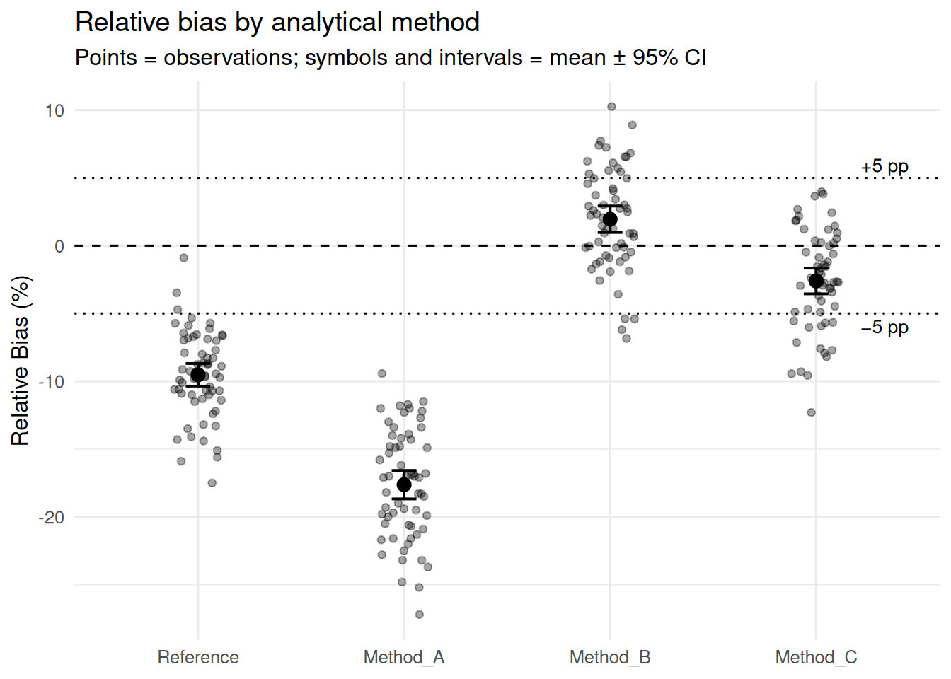
The estimated means are approximately:
Method
Mean relative bias
Reference
−9.5%
Method A
−17.7%
Method B
+2.0%
Method C
−2.6%
Several observations stand out.
Reference
The Reference method has a substantial negative bias.
This is important scientifically: the reference method is not assumed to be unbiased simply because it is called “Reference”.
Its performance is part of the problem we are investigating.
Method A
Method A is substantially more negatively biased than Reference.
The difference is large enough to be both statistically and chemically relevant.
Method B
Method B is closest to zero.
Its mean bias is approximately +2.0%.
Method C
Method C is also close to zero, at approximately −2.6%.
The estimated difference between B and C is therefore:
\[
2.0 - (-2.6)
\approx 4.6
\]
percentage points.
That is close to our 5-percentage-point threshold, but below it.
Whether that difference is statistically significant is a separate question from whether it is chemically relevant.
This distinction is precisely why we need to look beyond the global ANOVA p-value.
A simple analytical example
Suppose the true concentration of an analyte were 100 mg/kg.
A relative bias of −17.7% would correspond to an average result of approximately:
\[
100(1-0.177)=82.3\text{ mg/kg}
\]
The average difference would therefore be about 18 mg/kg.
A bias of this magnitude could be consequential when analytical results are compared with regulatory thresholds.
This does not mean that bias alone determines a regulatory decision.
Measurement uncertainty, the position of the result relative to the decision threshold and the applicable decision rule all matter.
The example simply illustrates why effect magnitude matters independently of statistical significance.
What assumptions have we made?
We have fitted a classical one-way ANOVA.
That means we have made assumptions about the error structure.
Independence
The observations contributing to the residual error should be independent, given the experimental design.
In our analytical scenario, each sample is homogenized and aliquoted, with separate aliquots analysed using the four methods.
For this dataset, we treat those analytical observations as independent replicates.
That assumption is based on the experimental process, not on a diagnostic plot.
This distinction matters.
Independence is fundamentally a property of how the observations were generated.
Later in the series we will examine situations involving shared batches, analysts, instruments or days, and consider when those sources of variation require a different model.
Normally distributed residuals
The classical F-test assumes normally distributed errors.
This does not mean that every group of raw observations must itself look perfectly normal.
The relevant assumption concerns the residuals of the fitted model.
Common residual variance
The classical model also assumes a common residual variance across the methods.
If one method is substantially more variable than another, the classical ANOVA inference may no longer have the properties we expect.
Again, we will investigate this properly later.
Why are we not checking every assumption now?
Because the purpose of this chapter is to understand the basic model and its global test.
A complete analysis of real data should not stop here.
But there is also a pedagogical danger in beginning with a long list of diagnostic tests before understanding what the model is doing.
So we will proceed incrementally.
For now:
state the assumptions;
understand why they matter;
fit the model;
interpret its result;
return to the assumptions later.
In Chapter 07 we will inspect residuals and diagnostics in detail.
In Chapter 08 we will deliberately violate important assumptions and investigate what happens to the inference.
What the ANOVA tells us — and what it does not
The global F-test has answered our first question.
It has not answered several other important questions.
1. Which methods differ?
The F-test tells us that the four population means are not all equal.
It does not tell us which pairs differ.
The coefficient table from lm() gives comparisons with Reference because of the chosen parameterization.
But perhaps the scientifically important comparison is B versus C.
That is not a reason to change the scientific question simply because R has chosen a convenient baseline.
It is a reason to formulate the appropriate comparison explicitly.
That is the subject of Chapter 02.
2. Does Matrix matter?
We deliberately ignored Matrix.
But the dataset contains three environmental matrices.
If the mean bias differs between Fill, Soil and Sediment, the one-way model is hiding potentially important structure.
We will introduce Matrix as a second factor in Chapter 03.
3. Does the effect of Method depend on Matrix?
This is a stronger question.
A method might perform well in one matrix and poorly in another.
If that happens, there may be no single method that can simply be labelled “best” independently of matrix.
This leads to interactions.
4. Is a statistically detectable difference chemically relevant?
ANOVA does not answer this.
The p-value concerns evidence against a statistical null hypothesis.
Chemical relevance requires a separate scientific criterion.
For this dataset, we have deliberately defined a 5-percentage-point threshold so that this distinction is concrete rather than merely theoretical.
One-way ANOVA is already more than a test
At first glance, the workflow seems almost trivial:
fit <-lm(RelativeBias_pct ~ Method, data = dat)anova(fit)
But those two lines hide several decisions.
We decided:
what the response variable should be;
what constitutes an observation;
which factor is relevant to the first question;
which structure to ignore temporarily;
what population-level hypothesis we want to test;
what error assumptions we are willing to make;
and what magnitude of effect would matter scientifically.
The function call is the easy part.
The statistical reasoning happened before it.
Take-home message
ANOVA is not a black box that outputs “significant” or “not significant”.
It is a linear model that compares variation between groups with variation within groups.
The F-test answers one specific global question:
Are the population means all equal?
For our dataset, the answer is clearly no.
But that is only the beginning.
We still need to determine:
which differences exist;
how large those differences are;
whether they are chemically relevant;
whether Matrix changes the picture;
whether Method and Matrix interact;
whether the model assumptions are defensible;
and eventually whether the model adequately represents the way the data were generated.
The statistical analysis becomes useful only when those questions remain connected to the scientific problem.
Next: Contrasts
We now know that the four methods do not have the same mean relative bias.
But the global F-test does not tell us which comparisons matter.
R has already produced three comparisons against the Reference method.
But are those the comparisons we actually want?
And what happens when we want to compare several methods while controlling the uncertainty associated with multiple comparisons?
Next, we move from the global ANOVA to contrasts and multiple comparisons.
The question becomes:
Which specific differences should we estimate, and how should we test them?