library(here)
library(data.table)
library(ggplot2)

dat <- fread(
  here("data", "dataset_v01_clean_balanced.csv")
)

dat[, Method := factor(
  Method,
  levels = c("Reference", "Method_A", "Method_B", "Method_C")
)]

dat[, Matrix := factor(
  Matrix,
  levels = c("Fill", "Soil", "Sediment")
)]

fit <- lm(
  RelativeBias_pct ~ Method * Matrix,
  data = dat
)07 — Diagnostics
Are the model assumptions defensible?
Scientific question
Every model we have fitted so far makes assumptions.
Some are mathematical assumptions about the distribution of the errors. Others are assumptions about how variability changes across the experimental conditions. One of them — independence — is fundamentally a property of the experimental design rather than something that can be repaired by a statistical test.
The question is therefore not:
“Did I get p < 0.05?”
Nor is it:
“Did all the diagnostic tests pass?”
The more useful question is:
“Are the assumptions of this model reasonable for this dataset, and would their violation threaten the conclusions we want to draw?”
This distinction matters because assumptions are rarely either perfectly satisfied or completely broken.
A model can be useful despite modest deviations from normality, for example. Conversely, a seemingly minor problem with independence can invalidate an otherwise impeccable ANOVA.
This chapter develops a practical diagnostic workflow for the interaction model used in Chapter 04.
The model
We return to the balanced dataset and fit the full two-way model:
\[ Y_{ijk} = \mu + \alpha_i + \beta_j + (\alpha\beta)_{ij} + \varepsilon_{ijk} \]
where:
- \(Y_{ijk}\) is the observed relative bias;
- \(\mu\) is the overall mean;
- \(\alpha_i\) is the effect of Method;
- \(\beta_j\) is the effect of Matrix;
- \((\alpha\beta)_{ij}\) is the Method × Matrix interaction;
- \(\varepsilon_{ijk}\) is the residual error.
For the classical ANOVA inference to be appropriate, we require the residuals to be approximately:
- independent;
- normally distributed;
- homoscedastic, with approximately constant variance;
- generated by a model whose systematic structure is correctly specified.
The last point is important.
A model can satisfy the distributional assumptions of linear regression and still be scientifically wrong.
Diagnostics therefore examine both the residual behaviour and the plausibility of the model structure.
Load the data and fit the model
For diagnostics it is useful to keep the fitted values and several types of residuals together with the original observations.
dat[, `:=`(
  fitted = fitted(fit),
  resid = residuals(fit),
  std_resid = rstandard(fit),
  student_resid = rstudent(fit),
  cooks = cooks.distance(fit)
)]
First diagnostic: residuals versus fitted values
The residuals-versus-fitted plot is usually the most informative first diagnostic.
It asks a simple question:
After accounting for the structure included in the model, is there still a systematic pattern left in the residuals?
Several patterns are particularly important.
- A curved pattern can indicate that the model has missed some systematic structure.
- A funnel shape can indicate non-constant variance.
- Clusters can indicate that an important grouping variable has been omitted.
- An isolated observation may deserve investigation as a potential outlier or influential point.
ggplot(dat, aes(x = fitted, y = resid)) +
  geom_point(alpha = 0.5, size = 2) +
  geom_hline(
    yintercept = 0,
    linetype = "dashed"
  ) +
  geom_smooth(
    method = "loess",
    se = TRUE,
    linewidth = 0.8
  ) +
  labs(
    x = "Fitted values",
    y = "Residuals",
    title = "Residuals vs Fitted"
  ) +
  theme_minimal(base_size = 12)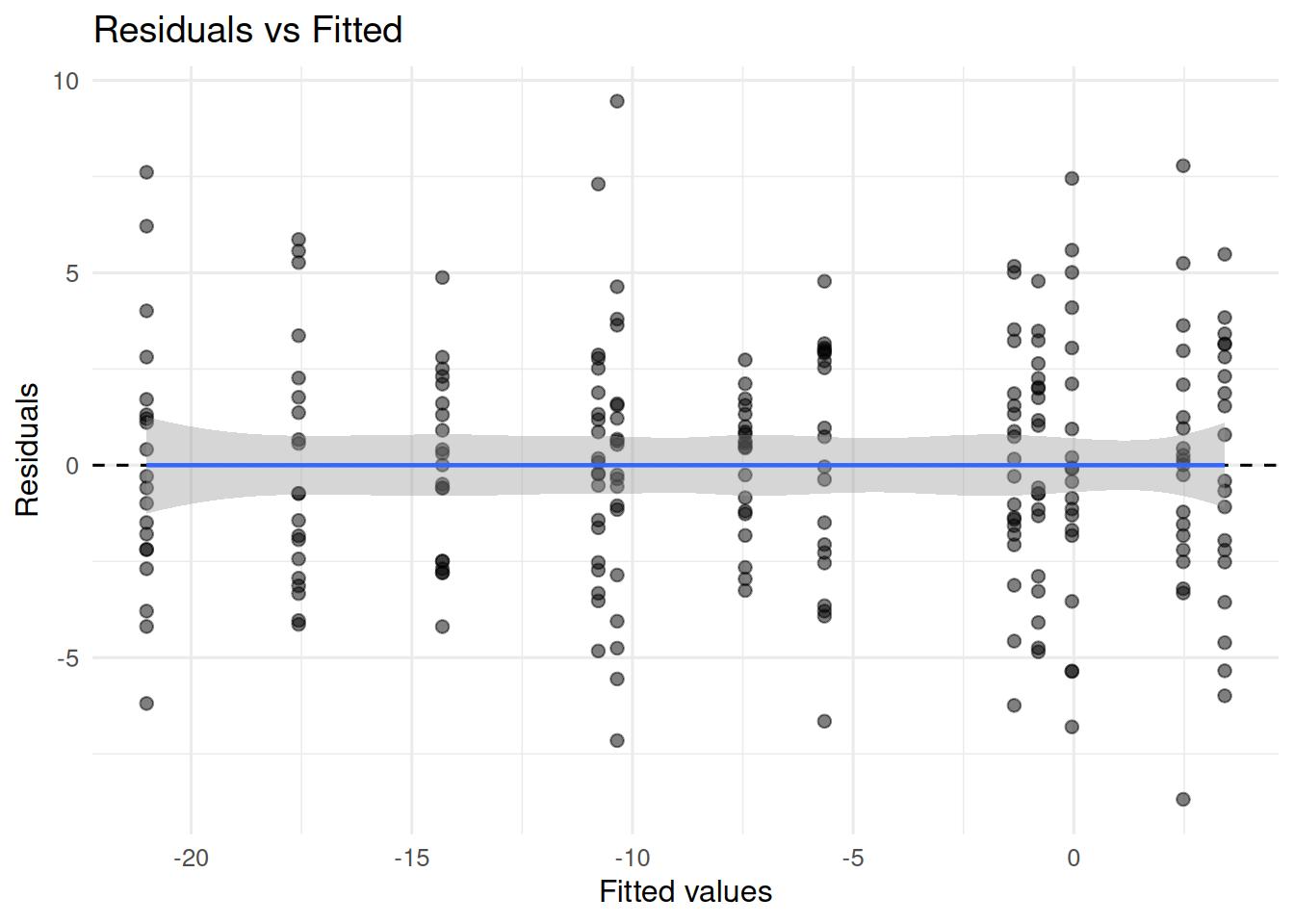
For our dataset, the residuals are reasonably scattered around zero.
There is no obvious curvature and no strong funnel-shaped pattern.
The smoother is approximately horizontal.
This is reassuring, but it is not a proof that the model is correct.
A residual plot can tell us that we do not see an obvious problem. It cannot prove that no relevant structure exists.
What does “constant variance” actually mean?
Homoscedasticity does not mean that every group must have exactly the same sample standard deviation.
It means that, under the model, the conditional variance of the response is assumed to be approximately constant after accounting for the predictors.
For our factorial model, this is a statement about the residual variability remaining after Method, Matrix and their interaction have been accounted for.
This distinction matters because looking only at the raw response can be misleading.
Two groups may have very different means but similar residual variance. Conversely, groups with similar means can have very different residual variance.
The residuals are therefore the appropriate scale on which to investigate this assumption.
Scale-location plot
The scale-location plot uses:
\[ \sqrt{|\text{standardized residual}|} \]
against the fitted values.
It is another way of looking for systematic changes in residual spread.
ggplot(
  dat,
  aes(x = fitted, y = sqrt(abs(std_resid)))
) +
  geom_point(alpha = 0.5, size = 2) +
  geom_smooth(
    method = "loess",
    se = TRUE,
    linewidth = 0.8
  ) +
  labs(
    x = "Fitted values",
    y = expression(sqrt("|Standardized residuals|")),
    title = "Scale-Location"
  ) +
  theme_minimal(base_size = 12)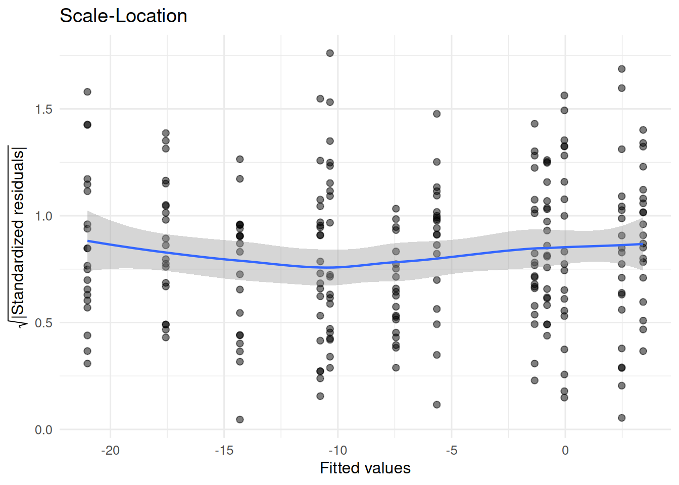
Again, the pattern is reasonably flat.
There is no strong indication that residual variability systematically increases or decreases with the fitted value.
This supports the assumption of approximately constant variance.
It is worth stressing the word approximately, as in real analytical data, exact equality of variances is neither expected nor necessary.
The relevant question is whether the departures are large enough to affect the inference we are making.
Normality of residuals
The normality assumption concerns the residual distribution, not the raw response variable.
This is an important distinction.
The response can be strongly non-normal because the experimental groups have different means. What matters for the classical linear-model inference is whether the residuals are reasonably compatible with the assumed error distribution.
We can inspect this using a normal Q-Q plot.
ggplot(dat, aes(sample = std_resid)) +
  stat_qq(alpha = 0.5, size = 2) +
  stat_qq_line(linewidth = 0.8) +
  labs(
    x = "Theoretical quantiles",
    y = "Standardized residuals",
    title = "Normal Q-Q"
  ) +
  theme_minimal(base_size = 12)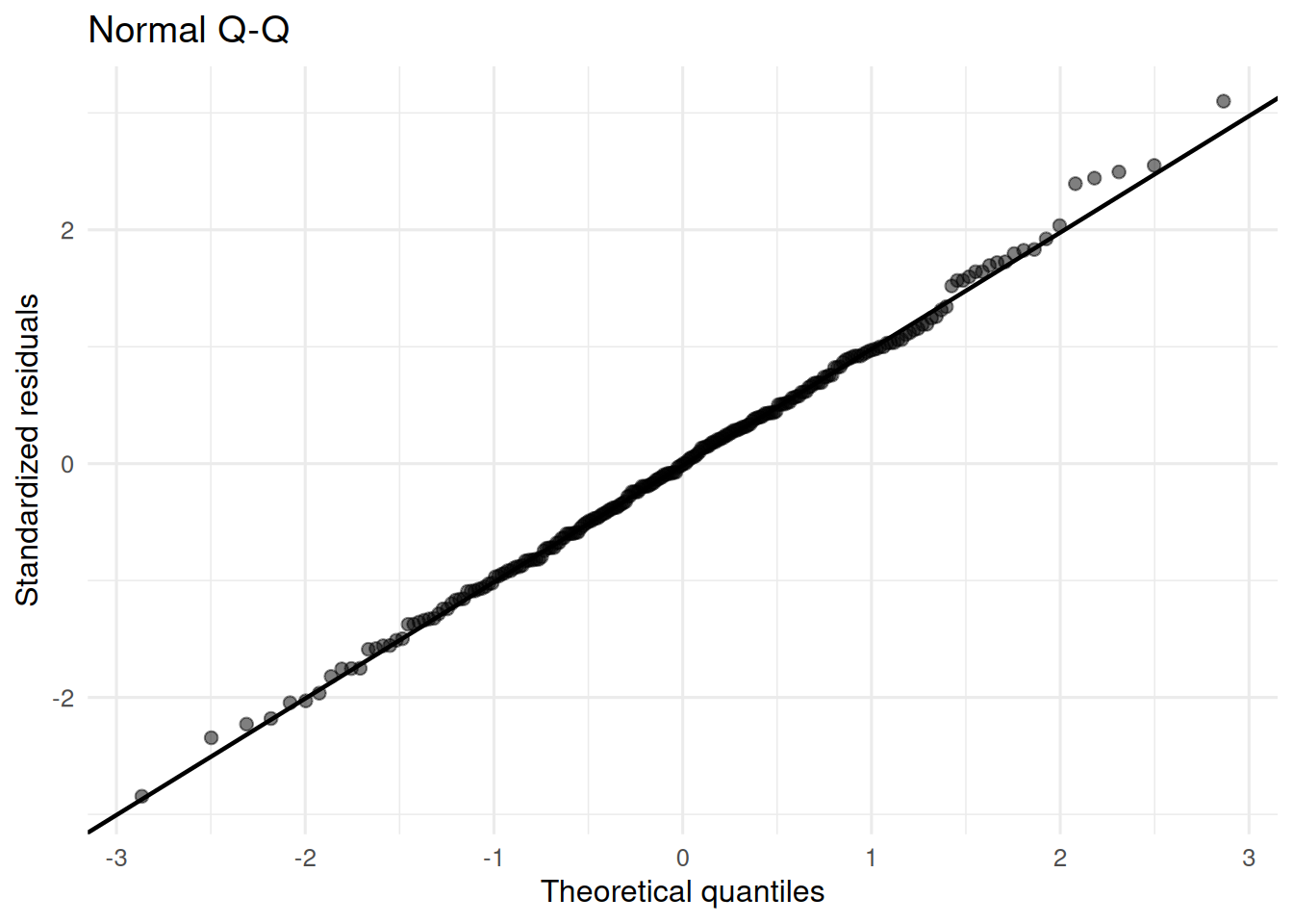
The points follow the reference line reasonably well.
There are some deviations in the tails, but no dramatic departure from normality.
For this dataset, the Q-Q plot therefore does not suggest a serious problem with the normal-error assumption.
Should we run Shapiro-Wilk?
A common workflow is:
- run Shapiro-Wilk;
- if \(p > 0.05\), declare normality;
- otherwise, abandon ANOVA.
This is not a good diagnostic strategy.
The Shapiro-Wilk test evaluates the null hypothesis that the sampled residuals are compatible with a normal distribution. It does not test whether the ANOVA is valid.
Its behaviour is also strongly dependent on sample size.
With enough observations, very small and practically irrelevant departures from normality can produce a small p-value.
With few observations, substantial departures may remain undetected.
We can nevertheless calculate it as a supplementary diagnostic:
shapiro.test(dat$resid)
    Shapiro-Wilk normality test

data:  dat$resid
W = 0.99773, p-value = 0.984
The result should be read together with the Q-Q plot, not as a pass/fail criterion.
A non-significant result does not prove normality.
A significant result does not automatically invalidate the model.
The useful question remains whether the observed deviation is large enough to threaten the inference we care about.
Homogeneity of variance: Levene’s test
A formal test can also be used to investigate whether residual variability differs across groups.
Levene’s test is often preferable to the classical Bartlett test because it is less sensitive to departures from normality.
For the factorial design, the natural grouping is the Method × Matrix combination.
library(car)

leveneTest(
  RelativeBias_pct ~ interaction(Method, Matrix),
  data = dat
)
Levene's Test for Homogeneity of Variance (center = median)
Df F value Pr(>F)
group 11 1.0811 0.3774
228 Again, the test should not be interpreted as a binary certification of homoscedasticity.
A non-significant result means that the data do not provide strong evidence against equal variances under the particular test.
It does not mean that the variances are exactly equal.
More importantly, the scientific question is not simply whether two variances are mathematically identical. We want to know whether the observed variance differences are large enough to alter the conclusions of the analysis.
Independence is different
Independence is often listed alongside normality and homoscedasticity as if it were another assumption that can be checked with a residual plot.
It is not.
Suppose the same environmental sample is analysed repeatedly. The measurements may be correlated because they share the same underlying material.
Suppose measurements are performed sequentially on the same instrument. Drift can create temporal correlation.
Suppose aliquots come from the same homogenised sample. Whether they can reasonably be treated as independent depends on the experimental context and on what source of variability the experiment is intended to represent.
No Shapiro-Wilk test can detect this.
No Levene test can repair it.
Independence must primarily be justified from the experimental design and measurement process.
For our dataset, each observation corresponds to a sample-method measurement and the design was constructed so that the observations entering this model can be treated as independent experimental units.
That assumption comes from how the dataset was generated, not from the fact that the residual plot looks acceptable.
This distinction becomes increasingly important as the series moves toward more complex experimental structures.
Residuals by experimental cell
Global diagnostic plots can hide problems affecting only one part of a factorial design.
For example, Method A might have much greater variability in Sediment while the other cells behave normally.
We therefore inspect residuals by Method and Matrix.
ggplot(
  dat,
  aes(x = Method, y = resid, fill = Matrix)
) +
  geom_boxplot(
    alpha = 0.6,
    outlier.shape = NA,
    position = position_dodge(0.8) # Assicura che i boxplot siano allineati
  ) +
  geom_jitter(
    position = position_jitterdodge(
      dodge.width = 0.8,     # Deve corrispondere alla larghezza del dodge dei boxplot
      jitter.width = 0.12    # La dispersione orizzontale dei punti
    ),
    alpha = 0.35,
    size = 1.2
  ) +
  geom_hline(
    yintercept = 0,
    linetype = "dashed"
  ) +
  labs(
    x = NULL,
    y = "Residuals",
    title = "Residuals by Method and Matrix"
  ) +
  theme_minimal(base_size = 12)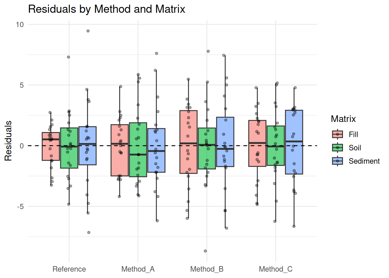
The residual distributions are broadly comparable across the cells.
There is no obvious cell with a substantially larger spread or a systematic displacement from zero.
This is consistent with the assumptions of the model.
It is also a useful reminder that diagnostics should respect the structure of the experiment.
Outliers and influential observations are not the same thing
An observation can be unusual without having a large effect on the fitted model.
Conversely, an observation that is not particularly extreme in absolute terms can be highly influential if it occurs in a part of the design where it has substantial leverage.
This distinction matters.
An outlier is unusual relative to the fitted model.
An influential observation is one whose presence materially changes the fitted model.
Cook’s distance is one way of investigating the latter.
ggplot(
  dat,
  aes(x = seq_along(cooks), y = cooks)
) +
  geom_col(alpha = 0.7) +
  geom_hline(
    yintercept = 4 / nrow(dat),
    linetype = "dashed"
  ) +
  labs(
    x = "Observation index",
    y = "Cook's distance",
    title = "Cook's Distance"
  ) +
  theme_minimal(base_size = 12)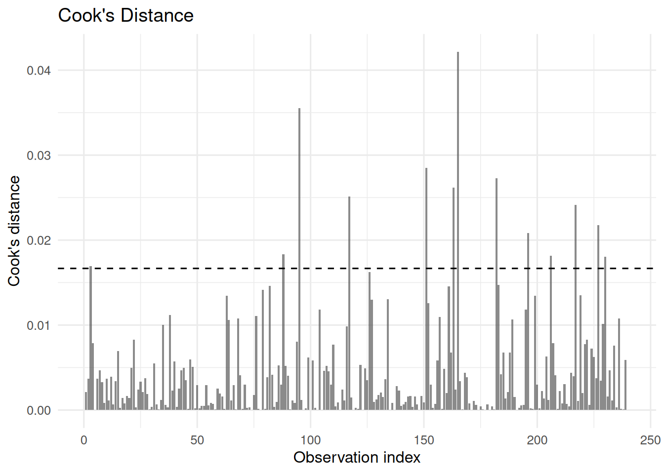
No observation has a Cook’s distance approaching 1.
A few observations may exceed the conventional reference value of \(4/n\), but this threshold is only a screening rule, not a definition of an influential observation.
An observation above \(4/n\) is not automatically bad.
The appropriate response is to investigate it.
Was there an analytical problem?
A transcription error?
A genuinely unusual sample?
Or simply a legitimate observation from the population of interest?
Removing observations solely because they influence the model is not a valid diagnostic strategy.
Diagnostics should be connected to the scientific question
Suppose we discover that Method A in Sediment has twice the residual variance of the other cells.
Does that automatically invalidate every conclusion?
No.
The consequence depends on what we want to estimate.
A variance problem may have relatively little effect on an estimated mean difference but substantially affect its standard error and therefore its confidence interval or p-value.
Likewise, a mild deviation from normality may have negligible consequences for a large balanced ANOVA but become important with very small samples or extreme heteroscedasticity.
This is why diagnostics cannot be reduced to a checklist.
The relevant question is always:
What part of my inference could this violation compromise?
Overall assessment
For the present dataset, the diagnostic evidence is reassuring:
- the residuals show no obvious systematic pattern;
- residual variance appears approximately constant;
- the Q-Q plot does not reveal severe non-normality;
- no cell shows an obvious residual pathology;
- there are no highly influential observations;
- independence is supported by the experimental construction rather than by a statistical test.
The classical ANOVA inference therefore appears defensible for this dataset.
But this conclusion is deliberately modest.
We have established that the model’s assumptions are reasonable, not that they are exactly true.
And we have not yet answered a more interesting question:
What happens when the assumptions are not reasonable?
That is the subject of the next episode.
Take-home message
Diagnostics are not a ritual performed before reporting p-values.
They are a way of asking whether the model is a credible representation of the data-generating process relevant to our scientific question.
Normality, homoscedasticity and influence can be investigated using residual diagnostics and supplementary formal tests.
Independence is fundamentally different: it must be justified by the experimental design.
Most importantly, an assumption violation is not automatically a command to abandon the analysis.
We need to understand which assumption is violated, how severely, and what consequence that violation has for the quantity we are trying to estimate.
That leads naturally to robustness.
Next: Robustness
The assumptions of our model look reasonable here, but real analytical datasets are rarely so cooperative.
What happens if variance becomes unequal?
What happens if a few observations become extreme?
What happens when the residual distribution departs substantially from normality?
And, perhaps most importantly:
Which of our conclusions survive when the assumptions behind the classical analysis are deliberately stressed?
Next, we perturb the dataset and compare alternative inferential approaches.