library(knitr)
source("R/create_dataset.R")Trying to Understand Variability in Extraction Yield
Why I started looking into mixed models
I did not start from mixed models.
I started from a practical concern in analytical chemistry:
how much of the variability I see is due to the method, and how much comes from the matrix?
More specifically:
am I overestimating the reliability of my results because I am treating dependent observations as independent?
The experiment
The goal is to study extraction yield of a compound.
We vary:
- extraction solvent
- temperature
And we measure:
- extraction yield
At first glance, this looks like a standard factorial experiment.
A limitation I initially ignored
At this point, there is an important detail in the experiment that I did not fully appreciate at the beginning.
Temperature is not applied within each soil.
Instead:
- some soils are only observed at low temperature
- others only at medium
- others only at high
This means that temperature and soil are structurally confounded.
In practice:
- each temperature level is associated with a specific subset of soils
- I never observe the same soil under different temperatures
So differences attributed to temperature may also reflect differences between soils. This is not a modeling issue. It is a limitation of the experimental design.
Interestingly, I found that the mixed model makes this limitation more visible. It cannot remove the confounding, but it reduces the apparent amount of information available for estimating temperature effects.
What makes this experiment different
The samples are not identical.
They come from different soil samples.
Each soil:
- has its own composition
- has its own organic content
- behaves differently during extraction
Within each soil sample:
- we apply different solvents
- we take replicate measurements
temperature is not varied within soil in this experiment
So the structure is:
- Soil sample / Temperature → Solvent → Replicates
The data
dataset <- create_dataset()
knitr::kable(dataset)| Soil | Temp | Solvent | Rep | Yield |
|---|---|---|---|---|
| S1 | Low | A | 1 | 52 |
| S1 | Low | A | 2 | 50 |
| S1 | Low | B | 1 | 55 |
| S1 | Low | B | 2 | 54 |
| S1 | Low | C | 1 | 57 |
| S1 | Low | C | 2 | 56 |
| S1 | Low | D | 1 | 53 |
| S1 | Low | D | 2 | 52 |
| S2 | Low | A | 1 | 48 |
| S2 | Low | A | 2 | 47 |
| S2 | Low | B | 1 | 51 |
| S2 | Low | B | 2 | 50 |
| S2 | Low | C | 1 | 52 |
| S2 | Low | C | 2 | 51 |
| S2 | Low | D | 1 | 49 |
| S2 | Low | D | 2 | 48 |
| S3 | Med | A | 1 | 60 |
| S3 | Med | A | 2 | 59 |
| S3 | Med | B | 1 | 63 |
| S3 | Med | B | 2 | 62 |
| S3 | Med | C | 1 | 65 |
| S3 | Med | C | 2 | 64 |
| S3 | Med | D | 1 | 61 |
| S3 | Med | D | 2 | 60 |
| S4 | Med | A | 1 | 57 |
| S4 | Med | A | 2 | 56 |
| S4 | Med | B | 1 | 59 |
| S4 | Med | B | 2 | 58 |
| S4 | Med | C | 1 | 61 |
| S4 | Med | C | 2 | 60 |
| S4 | Med | D | 1 | 58 |
| S4 | Med | D | 2 | 57 |
| S5 | High | A | 1 | 68 |
| S5 | High | A | 2 | 67 |
| S5 | High | B | 1 | 71 |
| S5 | High | B | 2 | 70 |
| S5 | High | C | 1 | 73 |
| S5 | High | C | 2 | 72 |
| S5 | High | D | 1 | 69 |
| S5 | High | D | 2 | 68 |
| S6 | High | A | 1 | 64 |
| S6 | High | A | 2 | 63 |
| S6 | High | B | 1 | 66 |
| S6 | High | B | 2 | 65 |
| S6 | High | C | 1 | 68 |
| S6 | High | C | 2 | 67 |
| S6 | High | D | 1 | 65 |
| S6 | High | D | 2 | 64 |
First observation
library(ggplot2)

ggplot(dataset, aes(x = Soil, y = Yield)) +
    geom_jitter(width = 0.1, alpha = 0.7) +
    labs(title = "Extraction yield by soil sample") +
    theme_minimal()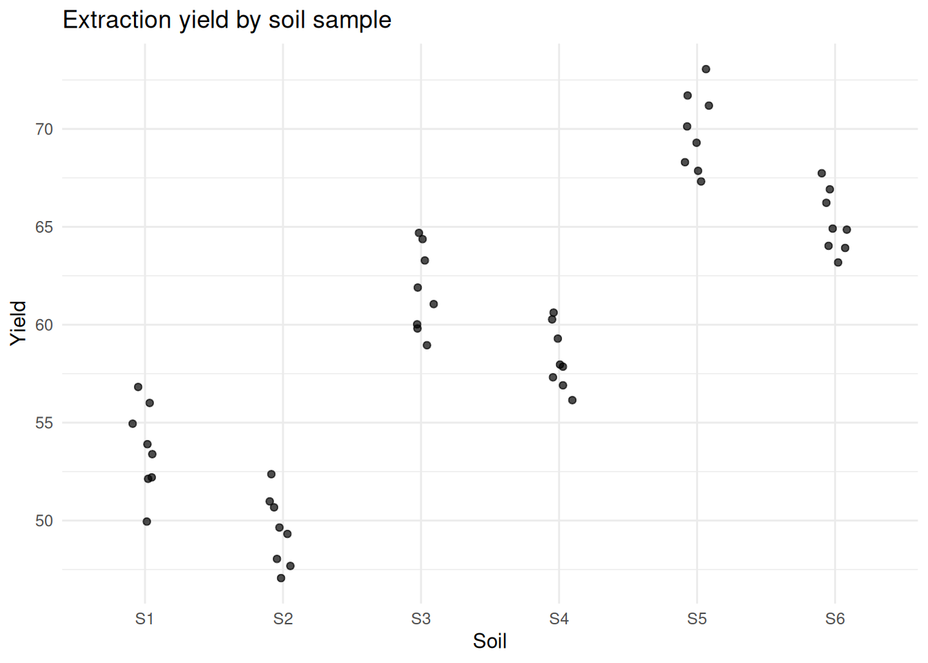
At this point, something becomes difficult to ignore.
Measurements from the same soil were consistently closer to each other than to measurements from other soils.
That was the first sign that I was not observing independent data points, but repeated observations of the same underlying systems.
A question that changed the analysis
are these observations independent?
Because if they are not:
- the model I use is misaligned
- the amount of information is overestimated
Looking at the variability more carefully
soil_means <- dataset[, .(mean_yield = mean(Yield)), by = Soil]

ggplot(dataset, aes(x = Soil, y = Yield)) +
    geom_point(alpha = 0.4) +
    geom_point(data = soil_means, aes(y = mean_yield), size = 3) +
    labs(title = "Within vs between soil variability") +
    theme_minimal()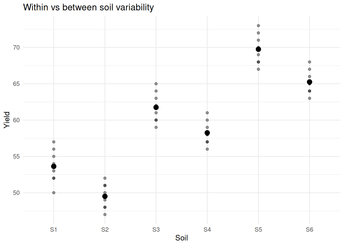
There are clearly two sources of variation:
- differences between soils
- differences within soils
What I was doing initially
m_naive <- lm(Yield ~ Temp + Solvent, data = dataset)
summary(m_naive)
Call:
lm(formula = Yield ~ Temp + Solvent, data = dataset)

Residuals:
    Min      1Q  Median      3Q     Max
-3.1458 -1.9948 -0.1771  2.0208  3.0208

Coefficients:
            Estimate Std. Error t value Pr(>|t|)
(Intercept)  65.3958     0.8009  81.650  < 2e-16 ***
TempLow     -15.9375     0.8009 -19.899  < 2e-16 ***
TempMed      -7.5000     0.8009  -9.364 7.68e-12 ***
SolventB      2.7500     0.9248   2.973  0.00486 **
SolventC      4.5833     0.9248   4.956 1.23e-05 ***
SolventD      1.0833     0.9248   1.171  0.24805
---
Signif. codes:  0 '***' 0.001 '**' 0.01 '*' 0.05 '.' 0.1 ' ' 1

Residual standard error: 2.265 on 42 degrees of freedom
Multiple R-squared:   0.91, Adjusted R-squared:  0.8993
F-statistic: 84.91 on 5 and 42 DF,  p-value: < 2.2e-16
This assumes:
- all observations are independent
- variability is homogeneous
At this point, that assumption no longer seems reasonable.
First correction: acknowledging structure
m_aov <- aov(Yield ~ Temp + Solvent + Error(Soil), data = dataset)
summary(m_aov)
Error: Soil
          Df Sum Sq Mean Sq F value Pr(>F)
Temp       2 2034.4    1017   15.41 0.0264 *
Residuals  3  198.1      66
---
Signif. codes:  0 '***' 0.001 '**' 0.01 '*' 0.05 '.' 0.1 ' ' 1

Error: Within
          Df Sum Sq Mean Sq F value Pr(>F)
Solvent    3 144.40   48.13   107.4 <2e-16 ***
Residuals 39  17.48    0.45
---
Signif. codes:  0 '***' 0.001 '**' 0.01 '*' 0.05 '.' 0.1 ' ' 1
This respects the experimental design.
But it mainly adjusts how tests are computed. It still does not parameterize variability as a quantity we can interpret.
Introducing a mixed model
Instead of asking: what is the correct test? I started asking: what generates these data?
To answer this question I tried to set up my fist mixel model.
library(lme4)
library(lmerTest)

m_lmer <- lmer(Yield ~ Temp + Solvent + (1 | Soil), data = dataset)
summary(m_lmer)
Linear mixed model fit by REML. t-tests use Satterthwaite's method [
lmerModLmerTest]
Formula: Yield ~ Temp + Solvent + (1 | Soil)
Data: dataset
REML criterion at convergence: 114.8
Scaled residuals:
Min 1Q Median 3Q Max
-2.25080 -0.64330 -0.06224 0.78819 1.35905
Random effects:
Groups Name Variance Std.Dev.
Soil (Intercept) 8.1966 2.8630
Residual 0.4482 0.6695
Number of obs: 48, groups: Soil, 6
Fixed effects:
Estimate Std. Error df t value Pr(>|t|)
(Intercept) 65.3958 2.0382 3.0409 32.085 5.99e-05 ***
TempLow -15.9375 2.8727 3.0000 -5.548 0.011548 *
TempMed -7.5000 2.8727 3.0000 -2.611 0.079633 .
SolventB 2.7500 0.2733 39.0000 10.062 2.15e-12 ***
SolventC 4.5833 0.2733 39.0000 16.770 < 2e-16 ***
SolventD 1.0833 0.2733 39.0000 3.964 0.000305 ***
---
Signif. codes: 0 '***' 0.001 '**' 0.01 '*' 0.05 '.' 0.1 ' ' 1
Correlation of Fixed Effects:
(Intr) TempLw TempMd SlvntB SlvntC
TempLow -0.705
TempMed -0.705 0.500
SolventB -0.067 0.000 0.000
SolventC -0.067 0.000 0.000 0.500
SolventD -0.067 0.000 0.000 0.500 0.500This is where the interpretation changes.
(1 | Soil) means:
- each soil has its own baseline
- these baselines vary
- that variability is estimated
Looking at the variability directly
vc <- VarCorr(m_lmer)

var_soil <- as.numeric(vc$Soil)
var_res  <- attr(vc, "sc")^2

var_soil
[1] 8.196582var_res[1] 0.4481838Now variability is explicit:
- between soils
- within soils
The estimation of similarity among samples within a soil can be calculated with intraclass correlation (ICC):
ICC <- var_soil / (var_soil + var_res)
ICC
[1] 0.9481555This can be interpreted as the proportion of total variance attributable to differences between soils. An ICC close to 1 means that observations within the same soil are very similar. Such high similarity within soils makes the confounding with temperature even more problematic.
In that case, adding more replicates within the same soil increases precision within that soil, but contributes very little to understanding variability across soils.
I was optimizing the wrong dimension of my experiment: replication instead of diversity.
Visualizing what remains within soils
dt_centered <- copy(dataset)
dt_centered[, centered := Yield - mean(Yield), by = Soil]

ggplot(dt_centered, aes(x = Soil, y = centered)) +
    geom_point(alpha = 0.6) +
    labs(title = "Within-soil variability after removing soil effects",
    y = "Mean centered yield") +
    theme_minimal()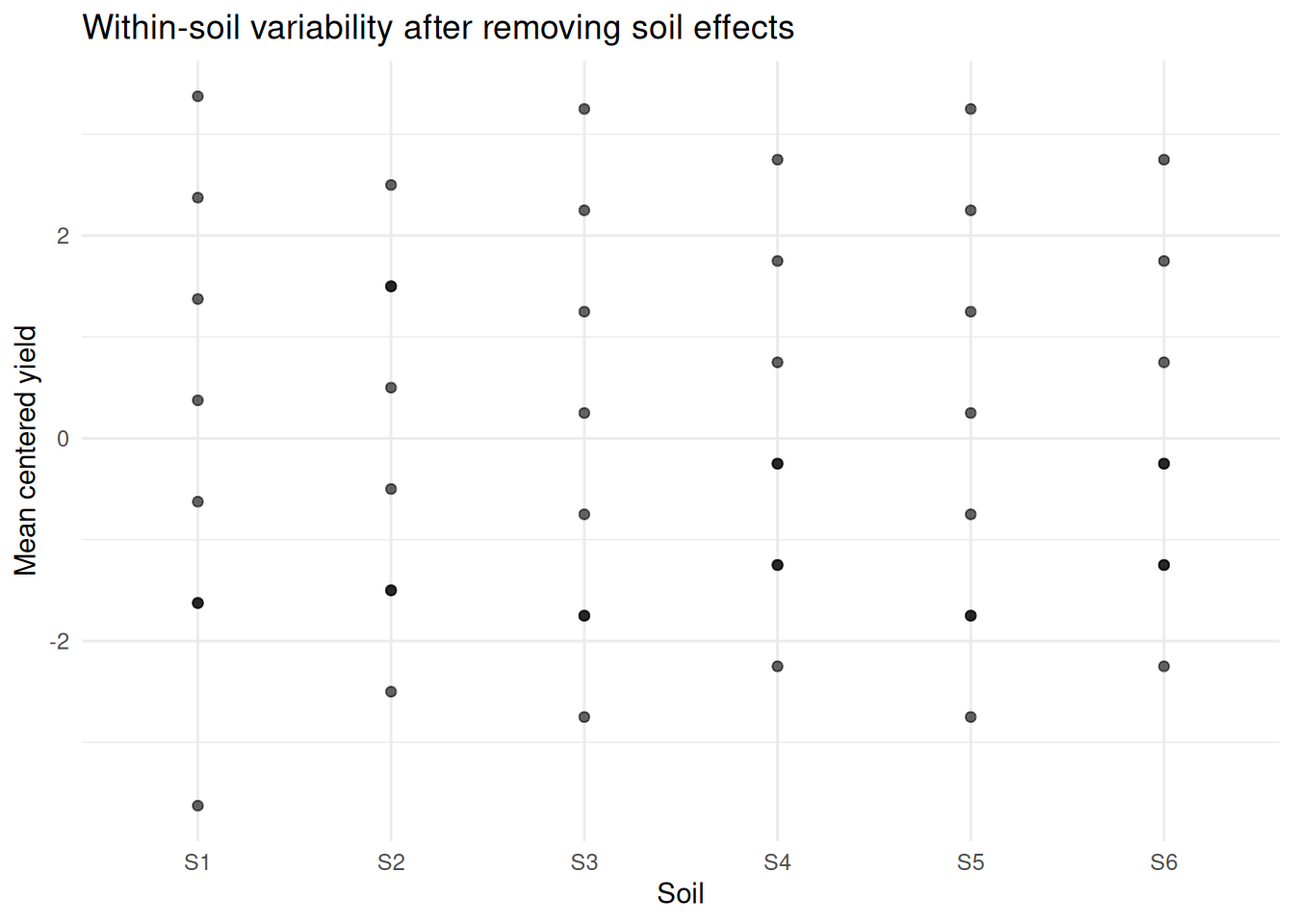
Most of the variation is removed when accounting for soil.
What I am actually estimating
I am not trying to compare these specific soils. I am trying to understand how much extraction yield would vary if I analyzed new soils.
This is a property of a population and it is estimated by a so called random effect.
To estimate a property of a population, I’m assuming:
- soils are representative
- there are enough of them
Otherwise the estimate of variability may not be reliable
Exploring uncertainty of the estimation
To explore this, I used a parametric bootstrap based on the fitted model. This generates new datasets consistent with the model assumptions, including the estimated variability between soils.
The resulting distribution shows that even variance estimates can be quite unstable with few groups.
set.seed(123)

boot_fun <- function(model) {
  as.numeric(VarCorr(model)$Soil)
}

boot_res <- bootMer(
  m_lmer,
  FUN = boot_fun,
  nsim = 200,
  use.u = TRUE,
  type = "parametric"
)ggplot(data.frame(var = boot_res$t), aes(x = var)) +
geom_histogram(bins = 20) +
labs(title = "Estimated variability between soils is itself uncertain") +
theme_minimal()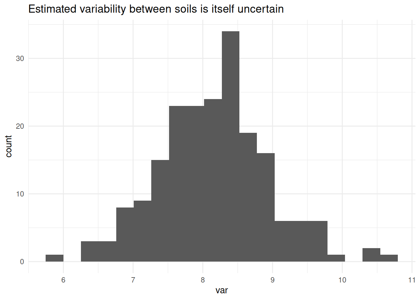
Implications for experimental design
If the goal is to understand variability across soils:
- adding more replicates within the same soil has diminishing returns
- adding more soils increases the amount of independent information
This was not obvious to me at the beginning.
What would happen if I ignored soil?
Up to this point, I have two possible models:
- A model that ignores soil structure (
m_naive) - A model that explicitly accounts for it (
m_lmer)
The question is: does it actually make a difference?
summary(m_naive)
Call:
lm(formula = Yield ~ Temp + Solvent, data = dataset)

Residuals:
    Min      1Q  Median      3Q     Max
-3.1458 -1.9948 -0.1771  2.0208  3.0208

Coefficients:
            Estimate Std. Error t value Pr(>|t|)
(Intercept)  65.3958     0.8009  81.650  < 2e-16 ***
TempLow     -15.9375     0.8009 -19.899  < 2e-16 ***
TempMed      -7.5000     0.8009  -9.364 7.68e-12 ***
SolventB      2.7500     0.9248   2.973  0.00486 **
SolventC      4.5833     0.9248   4.956 1.23e-05 ***
SolventD      1.0833     0.9248   1.171  0.24805
---
Signif. codes:  0 '***' 0.001 '**' 0.01 '*' 0.05 '.' 0.1 ' ' 1

Residual standard error: 2.265 on 42 degrees of freedom
Multiple R-squared:   0.91, Adjusted R-squared:  0.8993
F-statistic: 84.91 on 5 and 42 DF, p-value: < 2.2e-16summary(m_lmer)Linear mixed model fit by REML. t-tests use Satterthwaite's method [
lmerModLmerTest]
Formula: Yield ~ Temp + Solvent + (1 | Soil)
Data: dataset
REML criterion at convergence: 114.8
Scaled residuals:
Min 1Q Median 3Q Max
-2.25080 -0.64330 -0.06224 0.78819 1.35905
Random effects:
Groups Name Variance Std.Dev.
Soil (Intercept) 8.1966 2.8630
Residual 0.4482 0.6695
Number of obs: 48, groups: Soil, 6
Fixed effects:
Estimate Std. Error df t value Pr(>|t|)
(Intercept) 65.3958 2.0382 3.0409 32.085 5.99e-05 ***
TempLow -15.9375 2.8727 3.0000 -5.548 0.011548 *
TempMed -7.5000 2.8727 3.0000 -2.611 0.079633 .
SolventB 2.7500 0.2733 39.0000 10.062 2.15e-12 ***
SolventC 4.5833 0.2733 39.0000 16.770 < 2e-16 ***
SolventD 1.0833 0.2733 39.0000 3.964 0.000305 ***
---
Signif. codes: 0 '***' 0.001 '**' 0.01 '*' 0.05 '.' 0.1 ' ' 1
Correlation of Fixed Effects:
(Intr) TempLw TempMd SlvntB SlvntC
TempLow -0.705
TempMed -0.705 0.500
SolventB -0.067 0.000 0.000
SolventC -0.067 0.000 0.000 0.500
SolventD -0.067 0.000 0.000 0.500 0.500The two models are fitted on the same data, but they operate under different logic. While lm() treats all 48 rows as independent pieces of information, lmer() recognizes that observations are nested within soils.
For Solvent, we have 39 df. But for Temp, we have only 3.
Why? Because in this experimental design, temperature is a between-soil factor. Each soil was assigned to only one temperature. Since we have 6 soils and we are estimating 3 temperature levels, the model correctly identifies that we only have 6−3=3 independent units of information to compare temperatures.
If I use lm(), I am cheating: I am pretending I have 48 independent soils, which leads to overconfidence and artificially low p-values.
Looking at standard errors:
coef(summary(m_naive)) Estimate Std. Error t value Pr(>|t|)
(Intercept) 65.395833 0.8009326 81.649607 6.575338e-48
TempLow -15.937500 0.8009326 -19.898678 5.330250e-23
TempMed -7.500000 0.8009326 -9.364084 7.683805e-12
SolventB 2.750000 0.9248373 2.973496 4.860733e-03
SolventC 4.583333 0.9248373 4.955827 1.228580e-05
SolventD 1.083333 0.9248373 1.171377 2.480499e-01coef(summary(m_lmer)) Estimate Std. Error df t value Pr(>|t|)
(Intercept) 65.395833 2.0382134 3.040858 32.084881 5.993342e-05
TempLow -15.937500 2.8727347 3.000000 -5.547850 1.154772e-02
TempMed -7.500000 2.8727347 3.000000 -2.610753 7.963327e-02
SolventB 2.750000 0.2733081 39.000000 10.061906 2.147974e-12
SolventC 4.583333 0.2733081 39.000000 16.769844 1.993791e-19
SolventD 1.083333 0.2733081 39.000000 3.963781 3.051311e-04For Temperature: The model is more conservative. It recognizes that replicates within the same soil don’t provide new information about the effect of temperature — they only provide more precision about those specific 6 soils. It prevents us from attributing to temperature what may simply reflect differences between soils.
For Solvent: The model is actually more powerful. Because every solvent was tested on every soil (a within-soil comparison), the model can subtract the baseline variability of each soil. This isolates the solvent effect from the soil noise, making the standard error much smaller.
The mixed model isn’t just stricter. It is more aligned with the structure of the data. It reallocates power where it is earned (within-soil) and adds caution where it is needed (between-soil). Ignoring this structure doesn’t just change the numbers; it misrepresents the physical reality of the experiment.
A better version of the same experiment
After working through this example, I tried something simple.
I redesigned the experiment.
The goal was again understand how extraction yield depends on temperature and solvent, but I changed the experimental design.
In the original experiment each soil was observed at only one temperature. In the new version each soil is observed at all temperatures.
This removes the confounding between soil and temperature and Now temperature varies within soil, not only between soils, as happened with solvent in the previous design.
Creating a balanced experiment
dt_bal <- create_dataset_balanced()First, compare how temperature is distributed across soils.
dataset[, Experiment := "Confounded"]
dt_bal[, Experiment := "Balanced"]

dt_all <- rbind(dataset, dt_bal)

ggplot(dt_all, aes(x = Soil, y = Temp, color = Temp)) +
  geom_jitter(width = 0.1, height = 0.1, alpha = 0.7) +
  facet_wrap(~Experiment) +
  labs(title = "Temperature distribution across soils") +
  theme_minimal()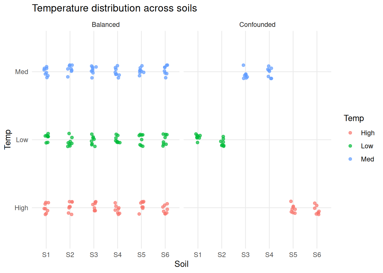
In the first experiment each soil appears at a single temperature. In the second each soil spans all temperatures. This is the key structural difference.
Now I can fit the two models and compare their standard error for the coefficients.
m_lmer_conf <- lmer(Yield ~ Temp + Solvent + (1 | Soil), data = dataset)
m_lmer_bal  <- lmer(Yield ~ Temp + Solvent + (1 | Soil), data = dt_bal)
se_conf <- coef(summary(m_lmer_conf))
se_bal <- coef(summary(m_lmer_bal))
se_conf_dt <- se_conf |> data.table() |> _[, Model := "Confounded"]
se_conf_bal <- se_bal |> data.table() |> _[, Model := "Balanced"]
se_all <- rbind(
data.table(term = rownames(se_conf), se = se_conf[, "Std. Error"], Model = "Confounded"),
data.table(term = rownames(se_bal), se = se_bal[, "Std. Error"], Model = "Balanced")
)
colnames(se_all) <- c("term", "se", "Model")
ggplot(se_all[grep("Temp", term)], aes(x = term, y = se, fill = Model)) +
geom_bar(stat = "identity", position = "dodge") +
labs(title = "Standard errors for temperature effects") +
theme_minimal()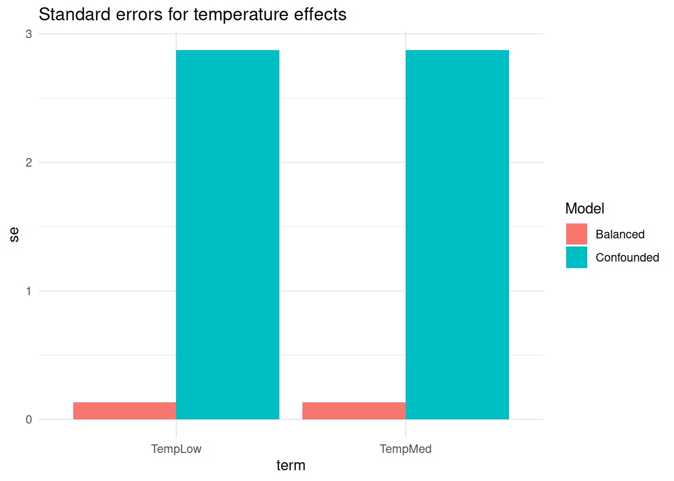
In the balanced experiment standard errors for temperature are smaller and uncertainty is reduced. This is not a consequence of a better model but of a better experimental design: now I have much more independent information available for estimating each effect.
In the first experiment temperature is estimated using differences between soils and very few independent units contribute.
In the second experiment temperature is estimated within each soil and many more comparisons are available.
In the balanced experiment:
- temperature effects are less entangled with soil differences
- estimates are more stable
- interpretation is more direct
Final takeaway
Mixed models were not a technical upgrade.
They became necessary because:
- the data were structured
- that structure mattered
- ignoring it changed the conclusions
- and some questions could not be answered given how the experiment was performed.
Mixed models, like any other statistical tools, cannot fix a badly designed experiment, but they can make its limitations visible.
What I am still trying to understand
- How many soil samples are enough?
- When does this variability start to affect decisions?
- When do these models change conclusions in practice?
- When is the added complexity actually justified?